面向高效实时分块的训练时动作条件化
Training-Time Action Conditioning for Efficient Real-Time Chunking
Kevin Black Allen Z. Ren Michael Equi Sergey Levine
Physical Intelligence
arXiv:2512.05964v2 [cs.RO],2025 年 12 月 9 日
Training-Time Action Conditioning for Efficient Real-Time Chunking
Kevin Black Allen Z. Ren Michael Equi Sergey Levine
Physical Intelligence
arXiv:2512.05964v2 [cs.RO],2025 年 12 月 9 日
目录
导读摘要(Abstract)1 引言(Introduction)2 相关工作(Related Work)3 预备知识(Preliminaries)4 训练时动作条件化(Training-Time Action Conditioning)5 实验(Experiments)5.1 仿真结果(Simulated Results)5.2 真实世界结果(Real-World Results)6 讨论与未来工作(Discussion and Future Work)7 致谢(Acknowledgments)8 附录:算法 1(Algorithm 1)参考文献(References)导读
要解决什么问题。 视觉-语言-动作模型(Vision-Language-Action model,VLA)动辄数十亿参数,一次推理要几十到上百毫秒,而机器人控制器通常以 50 Hz(每步 20 ms)运行。如果“等模型算完再动”,机器人就会一顿一顿的;如果边执行边推理,新生成的动作块又可能与正在执行的旧动作块衔接不上,产生突兀的“抖动”。作者此前提出的实时分块(Real-Time Chunking,RTC)通过推理时修补(inference-time inpainting)解决了衔接问题:生成新动作块时,把“推理期间必然还会执行的那几个旧动作”当作已知条件,让模型只“补全”其余部分。但这种修补依赖伪逆引导(pseudoinverse guidance),每个去噪步都要做一次反向传播求向量-雅可比积,额外增加了推理延迟,这恰恰与“实时”的初衷相悖。核心方法。 本文把“以动作前缀为条件”这件事从推理时挪到了训练时:训练时随机采样一个延迟 d,把真实动作块的前 d 个动作当作干净的、已知的前缀输入模型(其流匹配时间步设为 1,意思是“这些已经完全去噪了”),只对剩下的后缀加噪并计算损失。这样模型直接学会了条件分布 p(\mathbf{A}_{t+d:H}\mid\mathbf{o}_t,\mathbf{A}_{t:t+d})。推理时,只需每个去噪步把前缀覆盖回真实值即可,没有任何额外计算。实现上只需三处改动:允许每个动作 token 有各自的流匹配时间步、前缀用干净动作且时间步置 1、损失只算后缀。整个方法几行 JAX 代码即可实现(见文末算法 1)。主要结论。 (1)在 Kinetix 动态仿真基准上,延迟 d\ge 2 时训练时 RTC 的成功率高于推理时 RTC,延迟越大优势越明显;d=0,1 时略低一点点。(2)在真实世界的 \pi_{0.6} VLA 上做“折纸箱”和“做意式浓缩咖啡”两个复杂任务,训练时 RTC 的成功率和完成速度与推理时 RTC 持平(甚至成功率数值略高),而端到端延迟从约 135 ms 降到约 108 ms;两种 RTC 都明显快于同步推理基线。(3)代价是灵活性下降:只能用“硬”前缀,不能像推理时 RTC 那样对前缀之外的重叠动作做“软掩码”加权;还需要在训练时预先选好延迟的分布。需要的背景知识。- VLA:在预训练的视觉-语言模型(VLM)上增加动作输出能力,输入图像和语言指令,输出机器人动作。\pi_0、\pi_{0.5}、\pi_{0.6} 是 Physical Intelligence 的系列 VLA,其中由一个称为“动作专家”(action expert)的较小 Transformer 负责用流匹配生成连续动作。
- 动作分块(action chunking):策略一次预测未来 H 步的动作序列(一个“块”),而不是只预测下一步。好处是动作更平滑、能表达多模态行为、推理频率可以低于控制频率;坏处是块与块之间的衔接问题。
- 流匹配(flow matching):一种与扩散模型相近的生成模型训练方法。在噪声 \boldsymbol{\epsilon} 与数据 \mathbf{A} 之间做线性插值 \mathbf{A}^\tau=\tau\mathbf{A}+(1-\tau)\boldsymbol{\epsilon},训练网络预测“速度场”,生成时从纯噪声出发沿速度场积分(本文 \tau=0 为噪声、\tau=1 为数据)。
- 同步 / 异步执行:同步执行是执行完一个块的 s 步后停下来等下一次推理;异步执行是当前块还在执行时就开始算下一块。异步执行没有停顿,但新块生成时机器人已经往前走了 d 步。
- RTC 与推理时修补:RTC 在异步执行时,把推理延迟 d 期间必然执行的旧动作(前缀)“冻结”,用基于伪逆引导(\PiGDM)的修补方法让新块与之对齐。修补需要对网络求雅可比,代价较高。本文就是要用训练手段替代这一步。
- DiT 与 adaLN-zero:扩散 Transformer(Diffusion Transformer,DiT)用自适应层归一化(adaLN)把扩散/流匹配时间步注入网络:由时间步算出每层的缩放(scale)、平移(shift)和门控(gate)。本文的关键改动是让这些量按 token 区分。
摘要(Abstract)
原文
Real-time chunking (RTC) enables vision-language-action models (VLAs) to generate smooth, reactive robot trajectories by asynchronously predicting action chunks and conditioning on previously committed actions via inference-time inpainting. However, this inpainting method introduces computational overhead that increases inference latency. In this work, we propose a simple alternative: simulating inference delay at training time and conditioning on action prefixes directly, eliminating any inference-time overhead. Our method requires no modifications to the model architecture or robot runtime, and can be implemented with only a few additional lines of code. In simulated experiments, we find that training-time RTC outperforms inference-time RTC at higher inference delays. In real-world experiments on box building and espresso making tasks with the \pi_{0.6} VLA, we demonstrate that training-time RTC maintains both task performance and speed parity with inference-time RTC while being computationally cheaper. Our results suggest that training-time action conditioning is a practical drop-in replacement for inference-time inpainting in real-time robot control.
译文
实时分块(real-time chunking,RTC)通过异步地预测动作块(action chunk),并借助推理时修补(inference-time inpainting)以先前已提交的动作为条件,使视觉-语言-动作模型(vision-language-action model,VLA)能够生成平滑且反应灵敏的机器人轨迹。然而,这种修补方法会引入额外的计算开销,从而增加推理延迟。在本工作中,我们提出一种简单的替代方案:在训练时模拟推理延迟,并直接以动作前缀(action prefix)为条件,从而消除任何推理时开销。我们的方法无需修改模型架构或机器人运行时(runtime),只需额外几行代码即可实现。在仿真实验中,我们发现训练时 RTC 在较高推理延迟下优于推理时 RTC。在使用 \pi_{0.6} VLA 完成折纸箱和制作意式浓缩咖啡任务的真实世界实验中,我们证明训练时 RTC 在任务表现和速度上都与推理时 RTC 持平,同时计算代价更低。我们的结果表明,在实时机器人控制中,训练时动作条件化是推理时修补的一种实用的、可直接替换(drop-in)的方案。
解释
摘要按“背景—问题—方法—结果—结论”展开。
- 背景:RTC 是作者团队此前的工作,它让大模型在“边动边想”时依然平滑。所谓“以先前已提交的动作为条件”,是指在新动作块算出来之前,机器人肯定还要继续执行旧块里的若干动作,这些动作已经“定下来了”,新块必须与它们接得上。
- 问题:RTC 用“修补”实现这种约束,类似图像修补里“已知一部分像素,补全其余部分”。但它在推理时进行,需要额外的反向传播,于是推理变慢。为了实时性而引入的方法本身又拖慢了推理,这是本文要解决的矛盾。
- 方法:把条件化放到训练阶段。训练时随机假设“推理延迟为 d 步”,把真实动作的前 d 步直接作为输入告诉模型,让模型学会补全其余部分。
- 卖点:“drop-in replacement”指接口不变,可以直接替换原模块,不需要改机器人侧代码。
- 结果:仿真中高延迟时更好;真实机器人上表现持平但更省算力。
1引言(Introduction)
原文
Unlike chatbots or search engines, embodied agents must operate in real time. The feedback loop between an agent's actions and its environment necessitates reactivity — like a human athlete, an agent cannot simply “stop and think” while the outside world changes. However, the ever-increasing size of frontier models makes this more and more difficult. Nowhere is this more evident than in the domain of robot learning, where vision-language-action models (VLAs) consisting of billions of parameters have increasingly been used to control robots at high frequencies to accomplish dexterous tasks. Producing smooth yet reactive trajectories when the model inference latency is in the tens to hundreds of milliseconds is no small challenge.
译文
与聊天机器人或搜索引擎不同,具身智能体(embodied agent)必须实时运行。智能体的动作与环境之间的反馈回路要求它具备反应能力——就像人类运动员一样,当外部世界在变化时,智能体不能简单地“停下来思考”。然而,前沿模型的规模不断增大,使这一点越来越难做到。这一点在机器人学习领域表现得最为明显:由数十亿参数构成的视觉-语言-动作模型(VLA)正越来越多地被用于高频控制机器人以完成灵巧任务。当模型推理延迟在数十到数百毫秒量级时,生成既平滑又反应灵敏的轨迹绝非易事。
解释
这一段提出动机:物理世界不会等模型想完。聊天机器人慢一秒用户只是多等一会儿;机器人在倒咖啡、折纸箱时如果停下来“思考”,杯子里的液体、被按住的纸板都会继续运动,动作也会显得卡顿。给一个数量级的直觉:控制频率 50 Hz 意味着每 20 ms 就要输出一个动作;而一个数十亿参数的 VLA 推理一次需要 100 ms 左右,即约 5 个控制步。“平滑”(相邻动作不跳变)和“反应灵敏”(能快速利用新观测)在这里是一对矛盾:一次预测更长的动作序列可以更平滑,但对新观测的反应就更慢。
原文
Real-time chunking (RTC; [5]) presents an approach to this problem that combines action chunking [9, 27], flow matching [13], and inference-time inpainting [18, 21]. In RTC, action chunks are predicted asynchronously — the next chunk is generated while the current one is still executing. To ensure continuity between chunks, each generation is conditioned on a frozen prefix of previously predicted actions, inpainting the rest. However, the inference-time inpainting method used by RTC introduces additional computational overhead — and hence latency — that somewhat defeats the purpose of a real-time execution framework. Empirically, we also find that inference-time inpainting is fundamentally limited in its ability to handle high inference delays.
译文
实时分块(RTC;[5])为这一问题提供了一种方法,它结合了动作分块(action chunking)[9, 27]、流匹配(flow matching)[13] 和推理时修补 [18, 21]。在 RTC 中,动作块是异步预测的——当前块仍在执行时,下一个块就已在生成。为保证块与块之间的连续性,每次生成都以先前预测动作中一段被冻结的前缀为条件,并修补(补全)其余部分。然而,RTC 所用的推理时修补方法引入了额外的计算开销——因而也带来了延迟——这在某种程度上违背了实时执行框架的初衷。在实验中我们还发现,推理时修补在处理高推理延迟方面存在根本性的局限。
解释
这一段回顾 RTC 的三个组成部分,并指出它的两个缺点。
- 动作分块:一次输出一整段动作;流匹配:用来生成这段连续动作的生成模型;推理时修补:在生成过程中加入“前缀必须等于已知值”的约束。
- “冻结的前缀”:设推理从时刻 t 开始、耗时 d 步,那么在 t 到 t+d 之间机器人只能继续执行旧块中的动作。这 d 个动作已无法更改,新块也必须与它们一致,否则在 t+d 切换到新块时会出现跳变。
- 缺点一:开销。修补需要额外的反向传播,延迟变大。延迟变大又会使 d 变大,需要冻结的前缀变长,形成恶性循环。
- 缺点二:高延迟下效果下降。这一点在第 5.1 节的仿真实验中得到验证:前缀越长,基于线性化的修补越难做好。
原文
In this work, we augment RTC with an inpainting method that simulates inference delay at training time and eliminates any inference-time computational overhead. Our method works as a drop-in replacement for inference-time RTC: it requires no modifications to the model architecture or the robot runtime, and can be implemented with only a few additional lines of code. On simulated benchmarks, we find that training-time RTC outperforms inference-time RTC at higher inference delays. In the real world, we demonstrate that training-time RTC can be successfully added by fine-tuning a base model that was not pre-trained with action prefix conditioning. By applying training-time RTC to the \pi_{0.6} VLA [24], we show improved performance over inference-time RTC on two highly complex tasks: box building and espresso making.
译文
在本工作中,我们为 RTC 增加了一种修补方法:它在训练时模拟推理延迟,从而消除任何推理时计算开销。我们的方法可以直接替换推理时 RTC:它无需修改模型架构或机器人运行时,只需额外几行代码即可实现。在仿真基准上,我们发现训练时 RTC 在较高推理延迟下优于推理时 RTC。在真实世界中,我们证明可以通过微调一个未曾以动作前缀条件化方式预训练的基础模型,成功地加入训练时 RTC。通过将训练时 RTC 应用于 \pi_{0.6} VLA [24],我们在两个高度复杂的任务——折纸箱和制作意式浓缩咖啡——上展示了相对推理时 RTC 的性能提升。
解释
这一段是贡献总结,有三点值得注意。
- “模拟推理延迟”是全文的核心:训练数据中本来没有“延迟”的概念,作者人为随机选一个 d,假装前 d 个动作是已知的旧动作。
- “不需要从头预训练”:只需在已有基础模型上做任务微调时加入这一训练方式,因此对已经训练好的大模型很友好,实用价值高。
- 措辞差异:这里说“improved performance over inference-time RTC”,而摘要和第 5.2 节的说法是“parity”(持平)。从图 5 看,训练时 RTC 的成功率数值略高,但误差条有较大重叠,因此“持平”是更稳妥的解读。
2相关工作(Related Work)
原文
Action chunking and VLAs. Action chunking [9, 26] is the de facto standard in end-to-end imitation learning for visuomotor control. Recently, augmenting vision-language models (VLMs) to produce action chunks has demonstrated great success in robot manipulation, giving rise to vision-language-action models (VLAs) [4, 6–8, 10–12, 14, 17, 28, 29]. Subsequently, a plethora of methods have emerged to address the tension between large VLAs and high-frequency control. For example, Gemini Robotics [23] and GR00T [3] employ hierarchical VLA designs where the model is split into a heavyweight System 2 (high-level planning) and lightweight System 1 (low-level action generation) component. MiniVLA [2] and SmolVLA [20] present VLA architectures that are altogether faster and more efficient than most designs, making inference at the edge more feasible. These contributions are orthogonal to ours, and come with their own tradeoffs (e.g., modified network architectures and training recipes).
译文
动作分块与 VLA。动作分块 [9, 26] 是视觉运动控制(visuomotor control)端到端模仿学习中事实上的标准做法。近来,扩展视觉-语言模型(vision-language model,VLM)使其输出动作块的做法在机器人操作中取得了巨大成功,由此产生了视觉-语言-动作模型(VLA)[4, 6–8, 10–12, 14, 17, 28, 29]。随后,大量方法涌现出来,以缓解大型 VLA 与高频控制之间的矛盾。例如,Gemini Robotics [23] 和 GR00T [3] 采用分层 VLA 设计,把模型拆分为重量级的“系统 2”(System 2,高层规划)和轻量级的“系统 1”(System 1,底层动作生成)两部分。MiniVLA [2] 和 SmolVLA [20] 则提出了整体上比多数设计更快、更高效的 VLA 架构,使在边缘设备上推理更为可行。这些工作与我们的工作是正交的,并且有其各自的权衡(例如需要修改网络架构和训练方案)。
解释
这一段梳理“大模型 + 高频控制”这一矛盾的已有解法,可归为两类:
- 分层:借用认知科学里“系统 1 快思考 / 系统 2 慢思考”的说法。大模型低频地做规划,小模型高频地输出动作。这样快的部分很快,但要设计两套网络及其接口。
- 把模型做小:MiniVLA、SmolVLA 直接减少参数,代价是模型能力可能下降。
原文
Real-time execution of VLAs. The most closely related prior work is real-time chunking (RTC; [5]), which introduces an asynchronous execution framework that serves as a foundation for this work. Also related is SmolVLA [20], which presents an asynchronous execution algorithm that is similar to that of RTC; however, SmolVLA does not solve the inter-chunk discontinuity problem, which leads to out-of-distribution “jerks” between chunks. Concurrently to this work, A2C2 [19] and VLASH [22] both solve the discontinuity problem by adding a lightweight correction head and by conditioning on a single future action, respectively. In contrast to VLASH, we condition on a full prefix of future actions.
译文
VLA 的实时执行。与本文最密切相关的先前工作是实时分块(RTC;[5]),它提出了一个异步执行框架,也是本工作的基础。另一个相关工作是 SmolVLA [20],它提出了与 RTC 类似的异步执行算法;但 SmolVLA 没有解决块间不连续问题,这会在块与块之间造成分布外(out-of-distribution)的“急动”(jerk)。与本工作同期,A2C2 [19] 和 VLASH [22] 也都解决了不连续问题,分别通过增加一个轻量级修正头,以及以单个未来动作为条件来实现。与 VLASH 不同,我们以一段完整的未来动作前缀为条件。
解释
这一段与最直接的竞争方法做比较。
- SmolVLA 的异步执行:做到了“边执行边推理”,但新块与旧块之间没有约束,在切换时动作可能突然跳变。这种跳变在训练数据(人类示教)里从未出现过,所以是“分布外”的,机器人可能因此进入陌生状态,引发后续错误。
- A2C2:额外加一个小网络做修正,需要改架构。
- VLASH:思路与本文最接近,也是训练时条件化,但只以“单个”未来动作为条件;本文则以长度为 d 的整段前缀为条件,提供的信息更多(不仅是位置,还隐含了速度、加速度等运动趋势),衔接更平滑。
3预备知识(Preliminaries)
原文
We use the same problem formulation as RTC [5]: we begin with an action chunking policy denoted by p(\mathbf{A}_t\mid\mathbf{o}_t), where \mathbf{A}_t=[\mathbf{a}_t,\mathbf{a}_{t+1},\dots,\mathbf{a}_{t+H-1}] is a chunk of future actions, \mathbf{o}_t is an observation, and t indicates a controller timestep. We call H the prediction horizon, and at inference time, we roll out each chunk for s\le H timesteps, where s is the execution horizon.
译文
我们采用与 RTC [5] 相同的问题表述:从一个动作分块策略 p(\mathbf{A}_t\mid\mathbf{o}_t) 出发,其中 \mathbf{A}_t=[\mathbf{a}_t,\mathbf{a}_{t+1},\dots,\mathbf{a}_{t+H-1}] 是一个未来动作块,\mathbf{o}_t 是观测,t 表示控制器时间步。我们称 H 为预测视野(prediction horizon);在推理时,每个动作块只执行(rollout)s\le H 个时间步,s 称为执行视野(execution horizon)。
解释
这一段定义记号,后文所有内容都建立在这些符号之上。
- \mathbf{a}_t:时刻 t 的单步动作向量(例如双臂各关节的目标位置和夹爪开合,维度为 action_dim)。
- \mathbf{A}_t:从 t 开始的 H 个连续动作拼成的矩阵,形状为 H\times 动作维度。
- \mathbf{o}_t:时刻 t 的观测,例如多个相机的图像、机器人本体状态,以及语言指令。
- p(\mathbf{A}_t\mid\mathbf{o}_t):策略是一个条件分布而非确定性函数,因为同一个观测下人类示教可能有多种合理做法(多模态),所以用生成模型来表示。
- H 与 s:模型一次“想” H 步,但只“做”前 s 步,然后基于新观测重新规划。s 越小越接近闭环控制、反应越快;s 越大越依赖开环执行。例如在仿真实验中 H=8。
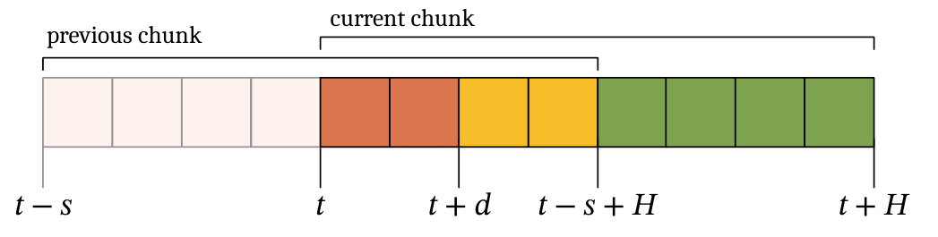
图 1
图 1 解读
画了什么:横轴是控制器时间步,每个小方格代表一个时间步的动作。上方两个括号分别标出“上一个块”(previous chunk,从 t-s 到 t-s+H)和“当前块”(current chunk,从 t 到 t+H)。图中示例取 H=8、s=4、d=2。各颜色含义:
- 浅粉色(t-s 到 t):上一个块中已经执行完的 s 个动作。上一个块在 t-s 时刻开始执行,执行了 s 步后到达 t,此时启动下一次推理。
- 红色(t 到 t+d):动作前缀。推理需要 d 步,这段时间里新块还没算出来,机器人只能继续执行上一个块中对应的动作,因此这些动作已“板上钉钉”,新块必须与之一致。
- 黄色(t+d 到 t-s+H):上一个块里还有、但会被新块取代的动作。它们不是硬约束,但作为“参考”能帮助新块平滑衔接。推理时 RTC 用指数递减的权重对它们做软约束(soft masking),训练时 RTC 则不使用。
- 绿色(t-s+H 到 t+H):上一个块没有覆盖的区域,完全由新块自由生成。
原文
To account for model inference, we define the quantity d to be the inference delay in units of controller timesteps. If inference begins at step t, then the resulting action chunk will not be available until step t+d, and so the first d actions cannot actually be executed. However, so long as d\le H-s, these first d timesteps will correspond to actions from the previous chunk that can be executed in the meantime. We call these d actions from the previous chunk that overlap with the current chunk the action prefix (see Figure 1).
译文
为了刻画模型推理,我们定义量 d 为以控制器时间步为单位的推理延迟(inference delay)。如果推理在第 t 步开始,那么得到的动作块要到第 t+d 步才可用,因此其前 d 个动作实际上无法执行。不过,只要 d\le H-s,这前 d 个时间步就对应着上一个块中的动作,可以在此期间执行。我们把上一个块中与当前块重叠的这 d 个动作称为动作前缀(action prefix,见图 1)。
解释
这一段把“推理延迟”量化为整数 d,并解释前缀的由来。换算示例:机器人控制频率 50 Hz(每步 20 ms),推理耗时 108 ms,则 d=\lceil 108/20\rceil\approx 5~6;论文写的是 d\approx 5。若推理耗时 135 ms,则 d\approx 7。关键直觉:新块的前 d 个动作“生成出来也没用”,因为对应的时间已经过去了。真正有用的是 \mathbf{A}_{t+d:H},它必须从前缀的末端“接着往下走”。如果模型不知道前缀是什么,它可能生成一个与前缀末端位置、速度都对不上的后缀,切换时就会出现急动。这正是 RTC(以及本文)以前缀为条件的根本原因。
原文
We consider policies trained with conditional flow matching [13], which minimizes the following loss:
\begin{aligned}\mathbf{A}_t^\tau &= \tau\mathbf{A}_t+(1-\tau)\boldsymbol{\epsilon}, \qquad \boldsymbol{\epsilon}\sim\mathcal{N}(\mathbf{0},\mathbf{I}) \end{aligned}(1)
\begin{aligned} \mathcal{L}(\theta) &= \mathbb{E}\,\big\|\mathbf{v}_\theta(\mathbf{A}_t^\tau,\mathbf{o}_t,\tau)-(\boldsymbol{\epsilon}-\mathbf{A}_t)\big\|^2 \end{aligned}(2)
where \mathbf{v}_\theta is a neural network and \tau denotes the flow matching timestep. At inference time, \mathbf{v}_\theta can be integrated from \tau=0 to 1 to produce samples from the dataset distribution p(\mathbf{A}_t\mid\mathbf{o}_t). 译文
我们考虑用条件流匹配(conditional flow matching)[13] 训练的策略,其最小化如下损失:
\begin{aligned}\mathbf{A}_t^\tau &= \tau\mathbf{A}_t+(1-\tau)\boldsymbol{\epsilon}, \qquad \boldsymbol{\epsilon}\sim\mathcal{N}(\mathbf{0},\mathbf{I}) &&(1)\\ \mathcal{L}(\theta) &= \mathbb{E}\,\big\|\mathbf{v}_\theta(\mathbf{A}_t^\tau,\mathbf{o}_t,\tau)-(\boldsymbol{\epsilon}-\mathbf{A}_t)\big\|^2 &&(2)\end{aligned}
其中 \mathbf{v}_\theta 是一个神经网络,\tau 表示流匹配时间步。在推理时,可以将 \mathbf{v}_\theta 从 \tau=0 积分到 1,从而得到服从数据集分布 p(\mathbf{A}_t\mid\mathbf{o}_t) 的样本。 解释
式 (1) 中各符号:
- \boldsymbol{\epsilon}:与动作块同形状的标准高斯噪声。
- \tau\in[0,1]:流匹配时间步(注意与控制器时间步 t 区分:t 是物理时间,\tau 是生成过程的“进度”)。\tau=0 时 \mathbf{A}^\tau_t=\boldsymbol{\epsilon} 是纯噪声,\tau=1 时 \mathbf{A}^\tau_t=\mathbf{A}_t 是干净的真实动作。
- \mathbf{A}^\tau_t:噪声和真实动作之间的线性插值,即“部分去噪”的动作。
- \mathbf{v}_\theta(\cdot):参数为 \theta 的网络(在 \pi_{0.6} 中就是“动作专家”),输入带噪动作、观测和 \tau,输出一个“速度”向量。
- 回归目标 \boldsymbol{\epsilon}-\mathbf{A}_t:对式 (1) 关于 \tau 求导得 \mathrm{d}\mathbf{A}^\tau_t/\mathrm{d}\tau=\mathbf{A}_t-\boldsymbol{\epsilon},即从噪声指向数据的速度。注意符号:论文正文写的是 (\boldsymbol{\epsilon}-\mathbf{A}_t),而算法 1 的代码里写的是
action_chunk - noise,即 \mathbf{A}_t-\boldsymbol{\epsilon};并且代码中采样时用x_t + dt * v_t从 \tau=0 积分到 1,这要求速度是 \mathbf{A}_t-\boldsymbol{\epsilon}。因此式 (2) 的符号应理解为一处笔误(或沿用了 \pi_0 中 \tau 方向相反的约定);以代码为准,网络学的是“从噪声走向数据”的方向。 - \mathbb{E}:对数据集中的 (\mathbf{o}_t,\mathbf{A}_t)、随机的 \tau 和 \boldsymbol{\epsilon} 取期望。
4训练时动作条件化(Training-Time Action Conditioning)
原文
Inference-time RTC [5] conditions the policy on the action prefix (Figure 1, red) using a inference-time inpainting method based on pseudoinverse guidance [18, 21]. For improved continuity between chunks, inference-time RTC additionally conditions on all overlapping actions, using exponentially decreasing weights for actions beyond the prefix (Figure 1, yellow). In RTC, this is referred to as “soft masking”. While pseudoinverse guidance affords great flexibility — enabling soft masking — it also requires computing a vector-Jacobian product (using backpropagation) during each denoising step.
译文
推理时 RTC [5] 使用一种基于伪逆引导(pseudoinverse guidance)[18, 21] 的推理时修补方法,使策略以动作前缀(图 1,红色)为条件。为了进一步改善块间连续性,推理时 RTC 还额外以全部重叠动作为条件,对前缀之外的动作(图 1,黄色)使用指数递减的权重。在 RTC 中,这被称为“软掩码”(soft masking)。伪逆引导虽然提供了很大的灵活性——使软掩码成为可能——但也要求在每个去噪步中计算一次向量-雅可比积(vector-Jacobian product,借助反向传播)。
解释
这一段说明原 RTC 是怎么做的,以及它为什么慢。伪逆引导的直觉:模型本来只会无条件地生成 \mathbf{A}_t。在去噪的第 \tau 步,模型可以“一步预测”出最终的干净动作 \hat{\mathbf{A}}^1。把它与已知前缀比较,得到误差;再通过反向传播算出“应该怎样微调当前带噪输入 \mathbf{A}^\tau,才能让 \hat{\mathbf{A}}^1 更接近前缀”,把这个修正量加到速度场上。这个“误差对输入求梯度”的操作就是向量-雅可比积:误差向量乘以网络输出对输入的雅可比矩阵。代价:每个去噪步都要多做一次反向传播。反向传播的计算量通常与前向传播同量级甚至更大,因此推理时间显著增加(实验中从 108 ms 增加到 135 ms)。软掩码:对红色前缀权重为 1(强约束),对黄色部分权重随时间指数衰减(越往后约束越弱),对绿色部分权重为 0。这让新块平滑地“过渡”到自己的规划上。这种按位置调节权重的灵活性是推理时方法独有的优点。
原文
The core insight of this work is that we can condition the policy on action prefixes at training time by simulating inference delay. While this does not afford the same flexibility as inference-time inpainting, it eliminates the computational overhead. Formally, we can learn p(\mathbf{A}_{t+d:H}\mid\mathbf{o}_t,\mathbf{A}_{t:t+d}), where \mathbf{A}_{t:t+d} is an action prefix (Figure 1, red) and \mathbf{A}_{t+d:H} is an action postfix (Figure 1, yellow and green), both taken from the same ground-truth action chunk. Implementing this for most standard policy architectures only requires 3 minimal changes:
译文
本工作的核心洞见是:我们可以通过模拟推理延迟,在训练时就让策略以动作前缀为条件。虽然这不具备推理时修补那样的灵活性,但它消除了计算开销。形式化地说,我们可以学习 p(\mathbf{A}_{t+d:H}\mid\mathbf{o}_t,\mathbf{A}_{t:t+d}),其中 \mathbf{A}_{t:t+d} 是动作前缀(图 1,红色),\mathbf{A}_{t+d:H} 是动作后缀(action postfix,图 1,黄色和绿色),二者都取自同一个真实动作块。对大多数标准策略架构而言,实现这一点只需要 3 处最小改动:
解释
符号说明:\mathbf{A}_{t:t+d} 是动作块中第 0 到第 d-1 个动作(即 \mathbf{a}_t,\dots,\mathbf{a}_{t+d-1});\mathbf{A}_{t+d:H} 是剩下的 H-d 个动作(下标中的 H 是块内索引的简写,严格说是到 t+H)。为什么可以这样做:训练数据是人类示教的连续轨迹,任意截取的一段 H 长动作都是平滑的。把它切成“前 d 个 + 后 H-d 个”,前者当作“已知的旧动作”,后者当作“要预测的新动作”,就构成了一个天然的监督样本,无需额外标注。模型学到的是“给定已经确定的开头,后面应该怎么接”。与修补的本质区别:修补是用一个无条件模型,在推理时近似地强加条件(依赖线性化,有近似误差);训练时条件化是直接学习条件分布(没有近似,但条件的形式在训练时就固定了)。这就是“灵活性换效率与精度”。一个微妙之处:训练时前缀来自真实轨迹,推理时前缀来自模型上一次的预测。只要模型的预测接近示教分布,这一差异就不大。
原文
- Modify the model architecture to allow for a different flow matching timestep for each action timestep. For a diffusion-transformer-like architecture [16], which uses adaLN-zero conditioning for the flow matching timestep, this is trivial — simply allow the scale, shift, and gate to differ between tokens. This does not change the number of learnable parameters.
- Use ground-truth, non-noisy actions for the prefix, and set the corresponding flow matching timesteps to 1. Do not change anything for the postfix. This conditions the model on the ground-truth action prefix while using it to denoise only the postfix.
- Mask the loss function so that loss is only computed on outputs corresponding to the postfix.
译文
- 修改模型架构,使每个动作时间步可以有不同的流匹配时间步。对于使用 adaLN-zero 条件化来注入流匹配时间步的类扩散 Transformer(diffusion transformer)架构 [16] 而言,这一点非常简单——只需允许缩放(scale)、平移(shift)和门控(gate)在不同 token 之间取不同值即可。这不会改变可学习参数的数量。
- 前缀使用真实的、无噪声的动作,并将其对应的流匹配时间步设为 1;后缀保持不变。这样模型就以真实动作前缀为条件,同时只用它来对后缀去噪。
- 对损失函数加掩码,使损失只在后缀对应的输出上计算。
解释
这三处改动是全文方法的全部内容,逐条解释如下。改动 1:逐 token 的时间步。在标准 DiT 中,时间步 \tau 经过一个小 MLP 得到每层的 (\gamma,\beta,\alpha)(scale、shift、gate),所有 token 共享同一组值:h\leftarrow h+\alpha\cdot f(\gamma\cdot\mathrm{LN}(h)+\beta)。现在把输入从一个标量 \tau 改为一个长度为 H 的向量 (\tau_0,\dots,\tau_{H-1}),同一个 MLP 对每个位置分别计算,得到逐 token 的 (\gamma_i,\beta_i,\alpha_i)。MLP 参数不变,只是批量地作用在更多输入上,所以参数量不变,这也是“无需修改模型架构”的含义(严格说是“不改参数”,前向计算的广播方式略有变化)。改动 2:前缀“已完成去噪”。把前缀 token 的 \tau 设为 1,在流匹配语义下等于告诉模型“这些 token 已经是干净数据了”。这样做的巧妙之处在于:
- 不需要额外的输入通道或特殊 token 来标记“这是前缀”,\tau=1 本身就是标记;
- 模型从各 token 的 \tau 分布中能直接读出延迟 d(有几个 1,d 就是几),图 2 的图注也指出了这一点;
- 当 d=0 时,所有 token 的 \tau 相同,退化为标准流匹配,因此兼容原模型的行为。
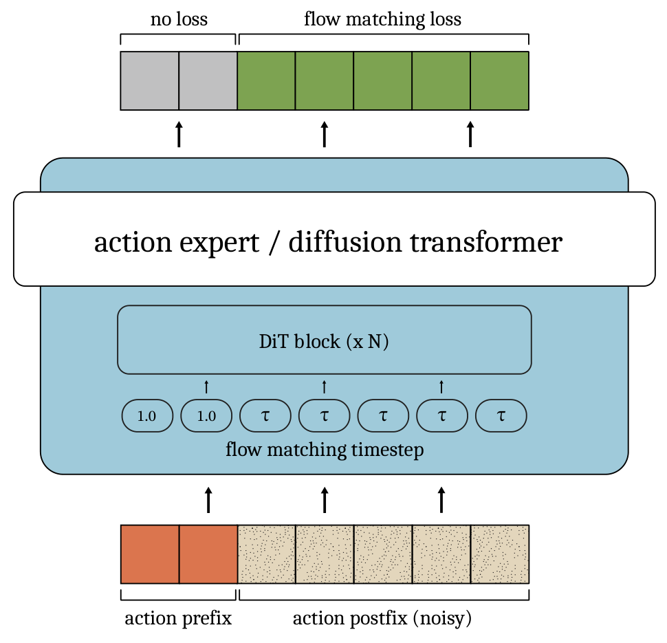
图 2
图 2 解读
自下而上读图:
- 底部输入:7 个动作 token。左边 2 个橙红色方块是动作前缀(干净的真实动作,此例中 d=2),右边 5 个带斑点的方块是带噪的动作后缀(斑点代表高斯噪声)。
- 中间蓝色大框:动作专家 / 扩散 Transformer,内部是 N 个 DiT 块。框内一排小圆角矩形是逐 token 的流匹配时间步:前缀两个为 1.0,后缀五个都是同一个 \tau。小箭头表示它们被送进 DiT 块(通过 adaLN-zero 调制)。
- 顶部输出:与输入一一对应的预测速度。前缀位置是灰色,标“no loss”(不计损失);后缀位置是绿色,标“flow matching loss”(计算流匹配损失)。
原文
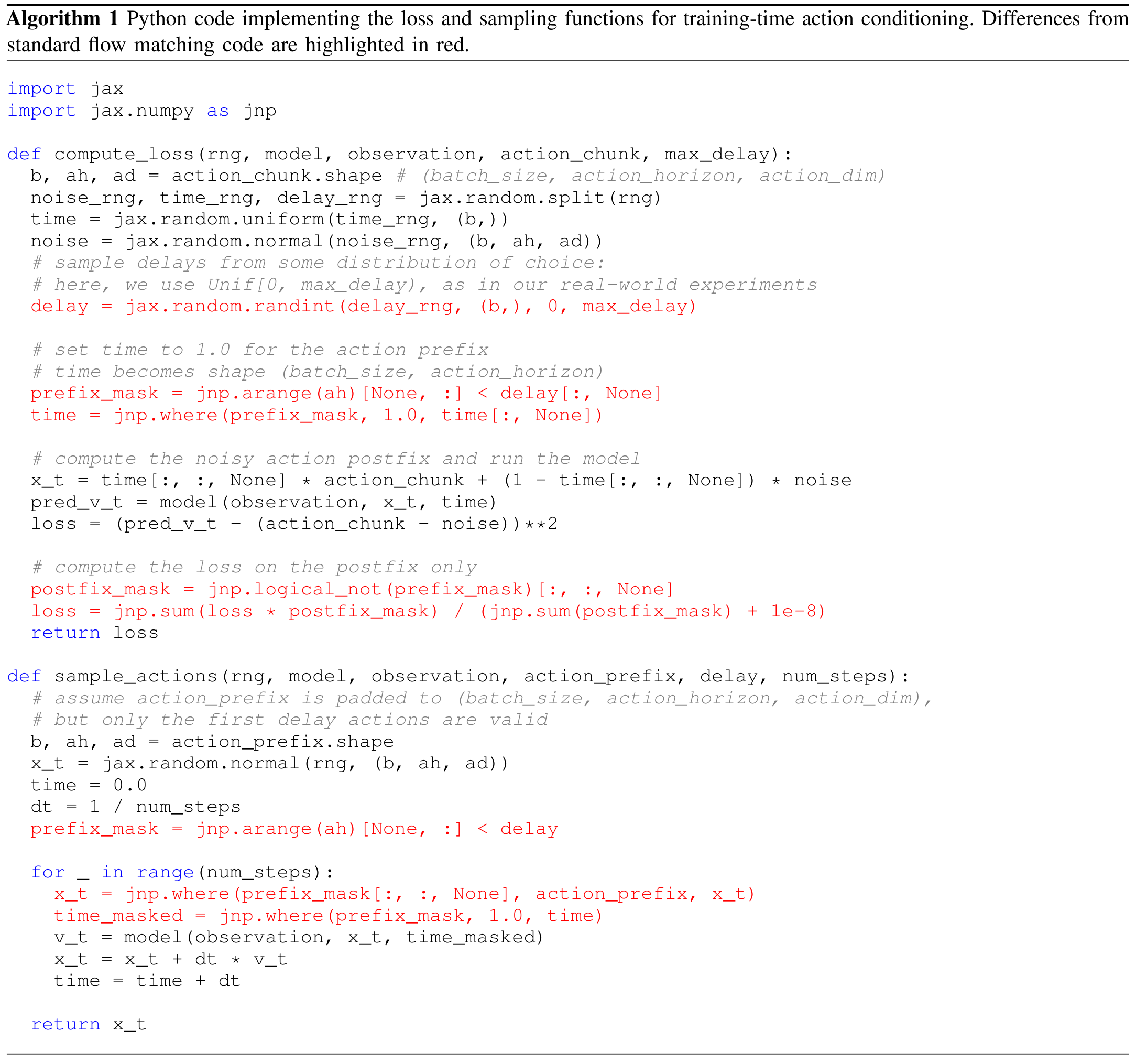
See Figure 2 for an illustration of this conditioning scheme as applied to a standard diffusion-transformer-like achitecture (e.g., the \pi_{0.6} action expert). See Algorithm 1 for Python code fully implementing loss calculation and action generation. In practice, since we do not know the exact inference delay ahead of time (and inference delays in the real world may vary), we sample d randomly during training.
译文
该条件化方案应用于标准类扩散 Transformer 架构(例如 \pi_{0.6} 的动作专家)的示意见图 2。完整实现损失计算和动作生成的 Python 代码见算法 1。在实践中,由于我们事先并不知道确切的推理延迟(而且真实世界中的推理延迟可能会波动),我们在训练时随机采样 d。
解释
为什么随机采样 d:真实部署中,网络传输、GPU 负载等都会让延迟波动(例如平均 108 ms,但有时 90 ms、有时 130 ms),对应的 d 也会在几个整数之间跳动。如果训练时固定 d=5,模型遇到 d=6 就是分布外输入。随机采样让一个模型能应对一段范围内的任意延迟。采样分布是一个超参数:仿真实验中采用指数递减的权重(偏向小 d),真实实验中采用 [0,10) 上的均匀分布。第 6 节也坦承,如何选这个分布是该方法的一个局限。算法 1 的完整代码及逐行解读放在第 8 节(原文位于论文最后一页)。
原文
With these modifications, action generation takes as input an action prefix \mathbf{A}_{t:t+d} and the delay itself d and produces as output an action postfix \mathbf{A}_{t+d:H}. As such, it adheres to the same interface as the action generation component of inference-time RTC (see [5], Algorithm 1) and thus acts as a seamless drop-in replacement.
译文
经过这些修改,动作生成以动作前缀 \mathbf{A}_{t:t+d} 和延迟 d 本身作为输入,并输出动作后缀 \mathbf{A}_{t+d:H}。因此,它与推理时 RTC 的动作生成组件(见 [5] 中的算法 1)遵循相同的接口,从而可以无缝地直接替换。
解释
这一段强调工程上的兼容性。原 RTC 系统中,机器人侧的运行时负责维护动作队列、测量延迟、在新块到达时切换;模型侧的“生成函数”只需满足“输入(观测, 前缀, d)\to 输出新块”这一签名。本文方法的签名与之完全一致,因此机器人侧代码一行都不用改,只要换一个微调过的模型权重和生成函数即可。这就是“drop-in replacement”的确切含义。
5实验(Experiments)
原文
In our experiments, we aim to compare training-time RTC to inference-time RTC, as well as to naive synchronous and asynchronous baselines. Our simulated experiments use the same dynamic Kinetix [15] benchmark as RTC (see [5] for details). Our real-world experiments build on the \pi_{0.6} base model [24], and include two precise and challenging tasks: box building and espresso making. We use the same experimental setup as \pi^*_{0.6} [1].
译文
在实验中,我们的目标是将训练时 RTC 与推理时 RTC 以及朴素的同步、异步基线进行比较。我们的仿真实验使用与 RTC 相同的动态 Kinetix [15] 基准(详见 [5])。我们的真实世界实验基于 \pi_{0.6} 基础模型 [24],包含两个要求精确且具有挑战性的任务:折纸箱和制作意式浓缩咖啡。我们使用与 \pi^*_{0.6} [1] 相同的实验设置。
解释
这一段交代参与比较的方法:
- 朴素同步(synchronous):执行完一个块后停下,等推理完成再继续,没有衔接问题,但每次都会停顿 d 步。
- 朴素异步(naive async):边执行边推理,新块到达后直接切换,不做任何前缀条件化,会出现块间跳变。
- 推理时 RTC:原方法,用伪逆引导修补。
- 训练时 RTC:本文方法。
5.1仿真结果(Simulated Results)
原文
In the dynamic Kinetix benchmark, following RTC [5], we train action chunking flow policies with a prediction horizon of H=8 and a 4-layer MLP-Mixer [25] architecture for 32 epochs on data generated by a mixture of expert policies. We report binary success rates with 2048 rollouts per data point and test delays between 0 (fully closed-loop) and 4 (the maximum supported when H=8). Naive asynchronous and inference-time RTC both use the same checkpoint, which is trained normally without action prefix conditioning for 32 epochs.
译文
在动态 Kinetix 基准中,我们遵循 RTC [5] 的做法,在由多个专家策略混合生成的数据上,用 4 层 MLP-Mixer [25] 架构训练预测视野 H=8 的动作分块流策略,共训练 32 个 epoch。我们报告二值成功率,每个数据点包含 2048 次 rollout,测试的延迟从 0(完全闭环)到 4(H=8 时支持的最大值)。朴素异步方法和推理时 RTC 使用同一个检查点(checkpoint),该检查点按常规方式训练 32 个 epoch,不使用动作前缀条件化。
解释
设置要点:
- MLP-Mixer:一种只用 MLP(无注意力)的架构,交替在 token 维和通道维做混合。这说明本文方法不局限于 Transformer,只要能接受逐 token 的时间步即可。
- 专家混合数据:用多个训练好的强化学习专家策略生成示教数据,因此数据是多模态的。
- “延迟 4 是最大值”:由图 1 的约束 d\le H-s 结合 s=\max(d,1) 得 d\le 8-d,即 d\le 4。
- d=0 为完全闭环:此时没有推理延迟,s=1,每一步都基于最新观测重新规划。
- 二值成功率:每次 rollout 只记成功(1)或失败(0),2048 次的平均即为成功率。
原文
For training-time RTC, we resume training from the 24th epoch and fine-tune for 8 epochs with action prefix conditioning. We do this so that all methods are matched in training compute. We sample delays from \{0,1,2,3,4\} with exponentially decreasing weights, as we found that higher delays need less training supervision. Better results could likely be obtained by spending more training compute training individual checkpoints for each delay.
译文
对于训练时 RTC,我们从第 24 个 epoch 恢复训练,并使用动作前缀条件化微调 8 个 epoch。这样做是为了让所有方法的训练计算量相同。我们以指数递减的权重从 \{0,1,2,3,4\} 中采样延迟,因为我们发现较高的延迟需要较少的训练监督。若投入更多训练计算、为每个延迟单独训练一个检查点,很可能得到更好的结果。
解释
公平比较的设计:24 + 8 = 32 个 epoch,与基线总训练量一致,排除了“多训练了一会儿所以更好”的可能。这也模拟了真实世界的用法:在已经常规训练好的模型基础上做条件化微调。为什么高延迟需要更少监督:延迟越大,前缀越长,模型需要预测的后缀越短(只有 H-d 个动作),任务越容易,而且前缀本身提供了大量信息。反之 d=0 时需要完整预测 8 个动作,最难。因此给小 d 更多采样权重是合理的。“每个延迟单独训练”:这里给出了提升空间——一个模型同时服务多个 d 会分摊容量,若部署时延迟已知且稳定,可以专门针对那个 d 训练。
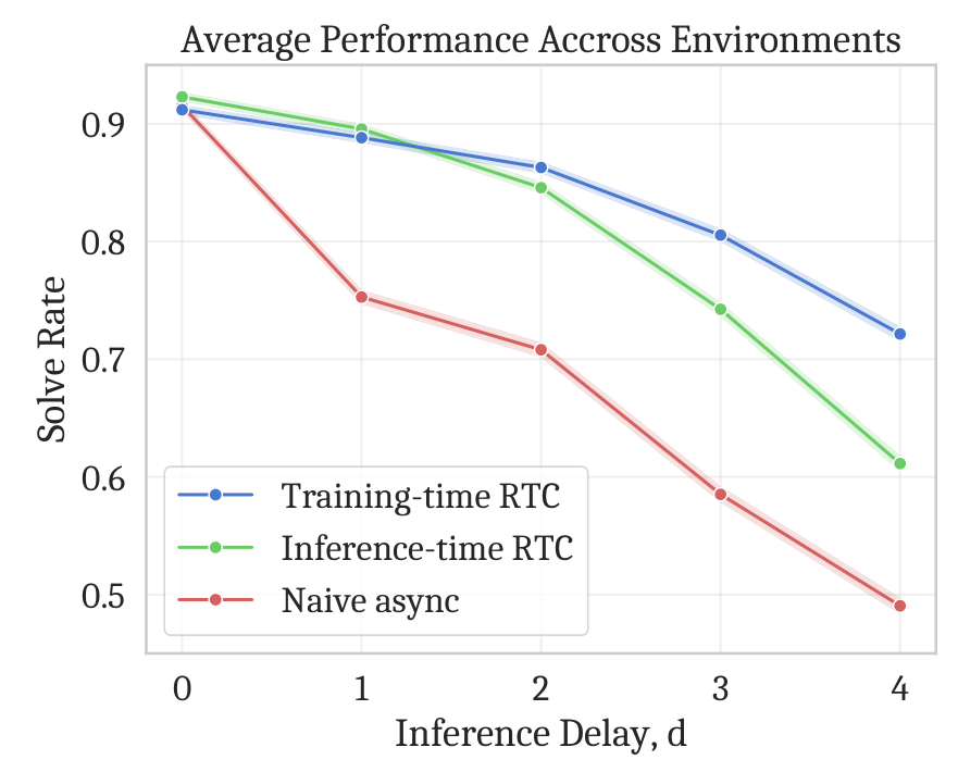
图 3
图 3 解读
坐标轴与图例:横轴是推理延迟 d(0–4 个控制步),纵轴是求解率(solve rate,即任务成功率),为所有 Kinetix 环境的平均值(图标题 “Average Performance Accross Environments” 中 Accross 为原图拼写错误,应为 Across)。三条曲线:蓝色为训练时 RTC,绿色为推理时 RTC,红色为朴素异步。阴影是 95% 置信区间;由于每点有 2048 次试验,区间很窄,几乎与线重合。关键数值(目测):
能读出的结论:
| 方法 | d=0 | d=1 | d=2 | d=3 | d=4 |
| 训练时 RTC | 0.91 | 0.89 | 0.86 | 0.81 | 0.72 |
| 推理时 RTC | 0.92 | 0.90 | 0.85 | 0.74 | 0.61 |
| 朴素异步 | 0.91 | 0.75 | 0.71 | 0.59 | 0.49 |
- d=0 时三者几乎相同:没有延迟就没有前缀,三种方法都退化为普通闭环控制。
- 朴素异步在 d=1 时就骤降约 16 个百分点,说明块间不连续的危害非常大,即便只延迟一步。
- 两种 RTC 在 d\le 1 时相当(推理时 RTC 略高约 1 个百分点);d=2 时训练时 RTC 开始反超;d=4 时领先约 11 个百分点(0.72 对 0.61)。差距随延迟扩大,这是本文在仿真中的核心证据。
- 所有方法都随 d 增大而下降,这是不可避免的:延迟越大,反应越慢,在动态环境中越容易失败。
原文
The results are presented in Figure 3. We find that training-time RTC outperforms inference-time RTC at inference delays of 2 and higher — with the gap significantly widening as the delay increases. This is likely because, as the size of the prefix grows, the inpainting algorithm has to “work harder” to produce a consistent postfix. In these cases, the training-time algorithm is more robust than the pure inference-time algorithm, which relies on a linearization obtained from the Jacobian of the model. Training-time RTC performs very marginally worse at delays of 1 and 0, likely because training-time RTC does not always receive training supervision for every action — i.e., slightly less training compute is spent learning to generate the first and second actions.
译文
结果见图 3。我们发现,在推理延迟为 2 及以上时,训练时 RTC 优于推理时 RTC——并且差距随着延迟增大而显著拉大。这很可能是因为随着前缀变长,修补算法必须“更加费力”才能生成一致的后缀。在这些情况下,训练时算法比纯推理时算法更加稳健,后者依赖于由模型雅可比矩阵得到的线性化。训练时 RTC 在延迟为 1 和 0 时表现略差,可能是因为训练时 RTC 并非总能对每个动作都获得训练监督——也就是说,用于学习生成第一个和第二个动作的训练计算略少。
解释
这一段给出两条原因分析。高延迟时为何训练时 RTC 更好:伪逆引导本质上是在当前点做一阶(线性)近似,用雅可比矩阵估计“改变输入会如何影响输出”,然后据此修正。前缀短时,所需的修正量小,线性近似足够准确;前缀长时,要让模型输出在很多个位置上同时匹配给定值,所需修正量大,线性近似失效,而且去噪步数有限(只有几步)来不及纠正。训练时方法则直接学习了条件分布,不涉及近似,因此更稳健。低延迟时为何略差:算法 1 中损失只在后缀上计算。如果训练时采样到 d=2,那么第 0、1 个动作就不计损失。整体来看,靠前位置的动作得到的训练信号比基线少,而 d=0 或 1 时恰恰需要模型生成这些靠前的动作。加上训练时 RTC 中有 8 个 epoch 被“分摊”给了不同的延迟,自然略逊于专门为 d=0 训练的模型。不过差距很小(约 1 个百分点)。
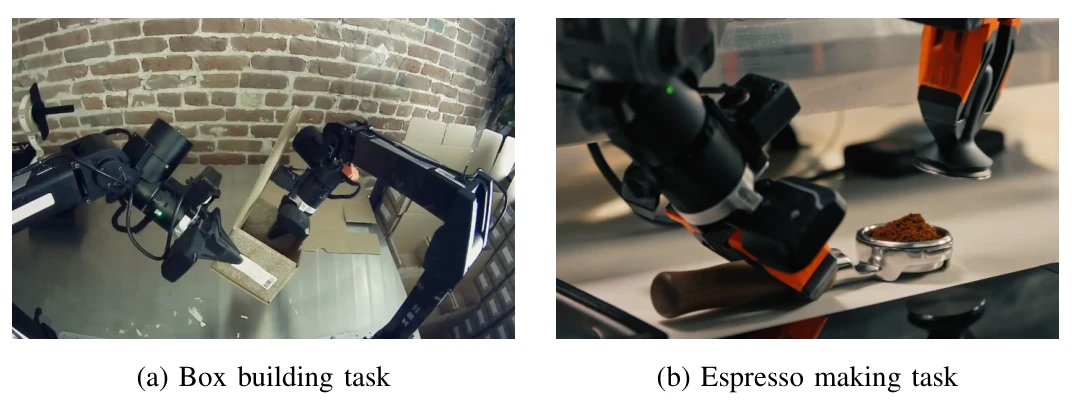
图 4
图 4 解读
(a) 折纸箱任务:两台机械臂(双臂平台)在桌面上将扁平纸板折成立体纸箱。需要双臂协作:一只手按住纸板,另一只手折叠侧翼,涉及可变形物体和较大的接触力,对动作的连续性要求很高,一旦动作突变就可能让纸板滑脱。(b) 意式浓缩咖啡任务:机械臂手持咖啡手柄(portafilter),图中手柄里装着咖啡粉。整个流程包括磨粉、压粉(tamping)、萃取、倒咖啡,是一个长时程、多阶段、需要毫米级精度的任务(例如手柄必须准确卡入咖啡机)。对论点的作用:这两个任务都是 \pi^*_{0.6} 论文中的代表性难任务,耗时长达 2–3 分钟,包含上千个控制步。选它们是为了证明方法在真实、复杂、长时程场景中同样可行,而不只是在玩具仿真中有效。这张图本身只是任务示意,不包含数据。
5.2真实世界结果(Real-World Results)
原文
In our real-world experiments, we use the \pi_{0.6} base model [24] and test on the espresso making and box building tasks from \pi^*_{0.6} [1]; see Figure 4 for an illustration. As in the simulated experiments, we use the same checkpoint for the synchronous baseline and inference-time RTC, and train a second checkpoint with action prefix conditioning for training-time RTC. Both checkpoints are fine-tuned from the base model on the target task for 8,000 gradient steps with a batch size of 512. We sample delays uniformly between 0 and 10 during training, which supports a maximum latency of 200ms on a 50Hz robot. During evaluations, we perform inference on a remote H100 server with 5 denoising steps, averaging 108ms of end-to-end latency for training-time RTC (d\approx 5) and 135ms for inference-time RTC (d\approx 7).
译文
在真实世界实验中,我们使用 \pi_{0.6} 基础模型 [24],并在来自 \pi^*_{0.6} [1] 的意式浓缩咖啡制作和折纸箱任务上进行测试;示意见图 4。与仿真实验一样,我们让同步基线和推理时 RTC 使用同一个检查点,并为训练时 RTC 另外训练一个带动作前缀条件化的检查点。两个检查点都从基础模型出发,在目标任务上以批大小 512 微调 8,000 个梯度步。训练时我们在 0 到 10 之间均匀采样延迟,这在 50 Hz 的机器人上可支持最高 200 ms 的延迟。评测时,我们在远程 H100 服务器上用 5 个去噪步进行推理,训练时 RTC 的平均端到端延迟为 108 ms(d\approx 5),推理时 RTC 为 135 ms(d\approx 7)。
解释
设置要点:
- 检查点数量:同步基线和推理时 RTC 共用常规微调的检查点,训练时 RTC 用带前缀条件化微调的检查点。两者训练步数和批大小一致,保证公平。
- 为什么是 200 ms:50 Hz 下每步 20 ms,d 最大约为 10,10\times 20=200 ms。代码中
randint(0, max_delay)是左闭右开区间,即实际采样 \{0,\dots,9\};论文描述为“0 到 10”,属于近似说法。 - 远程推理:模型在远程 GPU 服务器上运行,端到端延迟包括网络传输、图像编码、VLM 前向和动作专家去噪。
- 108 ms 对 135 ms:这 27 ms 的差距就是推理时 RTC 修补开销的直接体现(每个去噪步多一次反向传播,共 5 步)。换算成控制步,两种方法的 d 分别约为 5 和 7。值得注意的是,训练时 RTC 不仅更省算力,还因此获得了更小的 d,即对观测的反应更快。
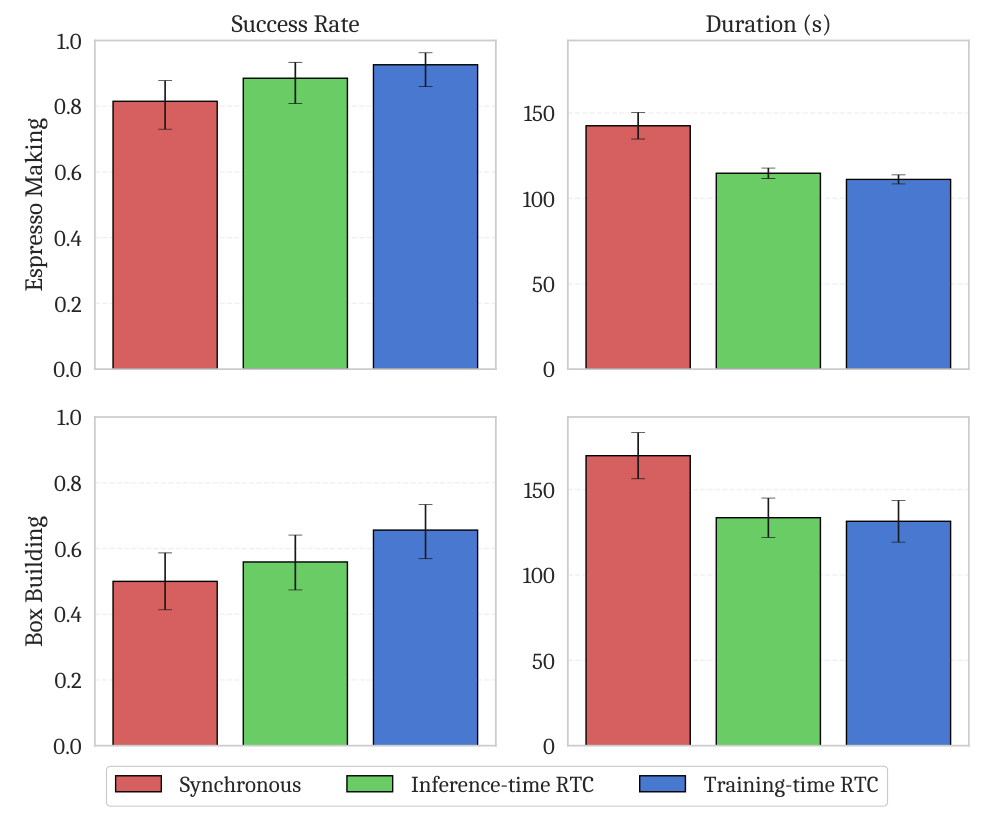
图 5
图 5 解读
版面结构:2\times 2 的柱状图。行对应任务(上:意式浓缩咖啡制作;下:折纸箱),列对应指标(左:成功率,越高越好;右:完成耗时,单位秒,越低越好)。颜色:红色为同步推理,绿色为推理时 RTC,蓝色为训练时 RTC。关键数值(目测):
能读出的结论:
| 意式浓缩咖啡 | 折纸箱 | |||
| 方法 | 成功率 | 耗时 (s) | 成功率 | 耗时 (s) |
| 同步 | \approx 0.81 | \approx 142 | \approx 0.50 | \approx 170 |
| 推理时 RTC | \approx 0.88 | \approx 115 | \approx 0.56 | \approx 133 |
| 训练时 RTC | \approx 0.92 | \approx 111 | \approx 0.66 | \approx 131 |
- 速度:两种 RTC 的耗时都比同步基线少约 20%(咖啡约少 30 秒,纸箱约少 40 秒),并且误差条与同步基线不重叠,差异明确。原因是同步执行在每个块之间都要停顿等待推理。
- 两种 RTC 之间:耗时几乎相同(训练时 RTC 略快),成功率训练时 RTC 数值上略高,但误差条明显重叠,统计上不能断言更好,所以作者在图注和正文中用了“表现相近 / 持平”的措辞。
- 成功率的误差条:用的是 68% 区间(约 \pm 1\sigma),比仿真图的 95% 区间更窄。这意味着即便 68% 区间重叠,也更不可能在 95% 水平上显著。读者应据此谨慎解读成功率差异。
- RTC 并未降低成功率:异步执行带来速度提升,同时没有牺牲甚至略微提高了成功率。
原文
The results are presented in Figure 5. We find that training-time RTC maintains both performance and speed parity with inference-time RTC without any computational overhead. Both variants of RTC clearly improve speed over the synchronous inference baseline, which exhibits visible pauses in between chunks.
译文
结果见图 5。我们发现,训练时 RTC 在没有任何计算开销的情况下,在性能和速度上都与推理时 RTC 持平。两种 RTC 变体都明显快于同步推理基线,后者在块与块之间会出现肉眼可见的停顿。
解释
这一段对图 5 做总结,措辞是“持平”(parity)而非“更优”,这是根据误差条做出的诚实判断。值得思考的一点:既然训练时 RTC 的延迟更低(d\approx5 对 d\approx7),为什么速度只是“持平”而没有明显更快?因为两种方法都是异步执行,机器人在推理期间不会停下,任务耗时主要取决于动作本身的执行速度,而不是推理快慢。延迟更低的好处主要体现在“反应性”上(新观测能更早地影响动作),这在高度动态的任务中更重要;在这两个以精确操作为主的任务里,效果不明显。同步基线的“肉眼可见的停顿”就是每个块执行完后等待约 100 ms 以上推理的结果,累积起来使总耗时增加约 20%。
6讨论与未来工作(Discussion and Future Work)
原文
In this work, we have presented a simple and effective drop-in replacement for real-time chunking (RTC) that elides any inference-time computational overhead by adding a small amount of additional training compute. Our method requires no modifications to the model architecture or the robot runtime, and can be implemented with only a few additional lines of code. Our simulated experiments show that training-time RTC outperforms inference-time RTC at higher inference delays, while our real-world experiments show that training-time RTC maintains both performance and speed parity with inference-time RTC without any computational overhead.
译文
在本工作中,我们提出了一种简单而有效的实时分块(RTC)直接替换方案:它通过增加少量额外的训练计算,省去了任何推理时计算开销。我们的方法无需修改模型架构或机器人运行时,只需额外几行代码即可实现。仿真实验表明,训练时 RTC 在较高推理延迟下优于推理时 RTC;真实世界实验则表明,训练时 RTC 在没有任何计算开销的情况下,在性能和速度上都与推理时 RTC 持平。
解释
这一段是全文总结,核心是一笔“交换”:把计算从推理阶段挪到训练阶段。训练只做一次,而推理在每次部署、每个控制周期都要执行,因此这种交换在工程上通常很划算。严格来说,“少量额外的训练计算”在实验中其实是“同等的训练计算”:仿真中总 epoch 数相同,真实实验中梯度步数相同。额外的部分仅在于“需要单独训练一个带条件化的检查点”,而不能直接复用常规训练的模型。
原文
However, training-time RTC is fundamentally less flexible than inference-time RTC; it only supports conditioning on a “hard” action prefix corresponding to the inference delay, whereas inference-time RTC can “softly” incorporate additional actions beyond the prefix. Additionally, training-time RTC requires carefully choosing the distribution of delays to simulate at training time based on the expected inference latency. We look forward to future work that can address these limitations and incorporate the best of both worlds.
译文
然而,训练时 RTC 从根本上不如推理时 RTC 灵活:它只支持以与推理延迟对应的“硬”动作前缀为条件,而推理时 RTC 可以“软性地”纳入前缀之外的更多动作。此外,训练时 RTC 需要根据预期的推理延迟,仔细选择训练时要模拟的延迟分布。我们期待未来的工作能够克服这些局限,兼取两者之长。
解释
作者坦承了两个局限:
- 无法软掩码:图 1 中的黄色区域(上一个块中前缀之后、仍有重叠的动作)被直接丢弃。这些动作虽不是硬约束,但能提供“上一次规划打算怎么走”的参考,有助于保持规划的一致性。训练时方法只能用 0/1 的硬掩码,无法表达“部分参考”。
- 延迟分布需预先设定:如果部署时的实际延迟超出训练时的采样范围(例如训练只覆盖 d<10,部署时网络变差导致 d=12),模型就会遇到分布外的输入。推理时 RTC 则没有这个问题,任何 d 都可以直接处理。
7致谢(Acknowledgments)
原文
We thank Laura Smith for developing the espresso making tasks, and helping with early evaluations. We thank Brian Ichter for feedback on the manuscript. As always, we thank our entire team of robot operators for their contributions to data collection and evaluations.
译文
我们感谢 Laura Smith 开发了意式浓缩咖啡制作任务并协助了早期评测。感谢 Brian Ichter 对本文稿提出的意见。一如既往,我们感谢整个机器人操作员团队在数据收集和评测方面的贡献。
解释
致谢部分没有技术内容。值得一提的是“机器人操作员团队”:真实世界的 VLA 研究高度依赖人工遥操作采集示教数据,以及人工执行大量评测试验(每个任务、每种方法都要跑数十次,每次 2–3 分钟),这是这类研究成本的主要来源之一。
8附录:算法 1(Algorithm 1)
算法 1
算法 1 解读
代码使用 JAX 编写,分为两个函数。以下按段落解读,并标出与标准流匹配的区别(即原图中的红色部分)。为便于对照,代码中的变量名用等宽字体书写。函数一:
compute_loss(训练损失) - 准备:从
action_chunk读出形状 (b, a_h, a_d),即批大小、动作视野 H、动作维度。把随机数种子拆成三份,分别用于噪声、时间步和延迟。为每个样本采样一个标量时间步 \tau\sim U[0,1],以及与动作块同形状的高斯噪声 \boldsymbol{\epsilon}。这部分与标准流匹配相同。 - [红] 采样延迟:
delay为每个样本从 [0,\texttt{max\_delay}) 中均匀采样一个整数。注释说明这里可以换成任何分布(例如仿真实验用的指数递减权重)。 - [红] 构造前缀掩码与逐 token 时间步:
prefix_mask形状为 (b,a_h),第 i 个位置为真当且仅当 i<d。随后用jnp.where把前缀位置的时间步改为 1.0,其余位置保持该样本的 \tau。于是time从形状 (b,) 变成 (b,a_h),对应改动 1 和改动 2。 - 加噪并前向:按式 (1) 计算 x_t=\tau\cdot\mathbf{A}+(1-\tau)\cdot\boldsymbol{\epsilon}。由于前缀位置 \tau=1,这一步自动得到干净的前缀,无需特殊处理,这正是“时间步设为 1”这个设计的巧妙之处。之后调用模型得到预测速度,并计算其与目标 \mathbf{A}-\boldsymbol{\epsilon} 的逐元素平方误差。
- [红] 只在后缀上算损失:
postfix_mask为前缀掩码取反,损失按掩码求和后除以有效元素个数(加 10^{-8} 防止除零)。对应改动 3。
sample_actions(推理采样) - 输入:
action_prefix被补齐为完整形状 (b,a_h,a_d),但只有前delay个动作有效(来自上一个动作块)。delay是实测的推理延迟 d。 - 初始化:x 从纯高斯噪声开始,\tau=0,步长 \delta=1/\texttt{num\_steps}(真实实验中为 5 步,\delta=0.2)。[红] 构造前缀掩码。
- 去噪循环,每一步:
- [红] 用真实前缀覆盖 x 的前 d 个位置,保证前缀始终是干净的已知值;
- [红] 前缀位置的时间步置 1.0,其余为当前 \tau;
- 调用模型得到速度 v,做一步欧拉积分 x\leftarrow x+\delta\cdot v,并令 \tau\leftarrow\tau+\delta。
- 输出:返回完整的 x。其前 d 个位置在最后一次欧拉更新中会被模型输出改动,因此并不严格等于前缀;但这部分本来就不会被执行,使用者只取后缀 x_{d:} 即可。
- 推理时每个去噪步只做一次普通前向,没有任何反向传播,这就是“零推理开销”的来源;与之对比,推理时 RTC 每步都要额外求一次向量-雅可比积。
- 红色代码总共不到 10 行,印证了“只需几行额外代码”的说法。
- 代码中的速度目标为 \mathbf{A}-\boldsymbol{\epsilon},与采样时从 \tau=0(噪声)积分到 \tau=1(数据)一致;正文式 (2) 写成 \boldsymbol{\epsilon}-\mathbf{A}_t,二者符号相反,以代码为准(见第 3 节式 (2) 的解释)。
- 训练函数中
delay形状为 (b,),每个样本延迟不同;采样函数中delay是标量,整批共用一个延迟,这符合部署时的实际情况。
参考文献(References)
参考文献按原文列出,未翻译。- Ali Amin, Raichelle Aniceto, Ashwin Balakrishna, Kevin Black, Ken Conley, Grace Connors, James Darpinian, Karan Dhabalia, Jared DiCarlo, Danny Driess, et al. \pi^*_{0.6}: a vla that learns from experience. arXiv preprint arXiv:2511.14759, 2025.
- Suneel Belkhale and Dorsa Sadigh. Minivla: A better vla with a smaller footprint, 2024. URL https://github.com/Stanford-ILIAD/openvla-mini.
- Johan Bjorck, Fernando Castañeda, Nikita Cherniadev, Xingye Da, Runyu Ding, Linxi Fan, Yu Fang, Dieter Fox, Fengyuan Hu, Spencer Huang, et al. Gr00t n1: An open foundation model for generalist humanoid robots. arXiv preprint arXiv:2503.14734, 2025.
- Kevin Black, Noah Brown, Danny Driess, Adnan Esmail, Michael Equi, Chelsea Finn, Niccolo Fusai, Lachy Groom, Karol Hausman, Brian Ichter, et al. \pi_0: A vision-language-action flow model for general robot control. arXiv preprint arXiv:2410.24164, 2024.
- Kevin Black, Manuel Y Galliker, and Sergey Levine. Real-time execution of action chunking flow policies. arXiv preprint arXiv:2506.07339, 2025.
- Anthony Brohan, Noah Brown, Justice Carbajal, Yevgen Chebotar, Xi Chen, Krzysztof Choromanski, Tianli Ding, Danny Driess, Avinava Dubey, Chelsea Finn, et al. Rt-2: Vision-language-action models transfer web knowledge to robotic control. In arXiv preprint arXiv:2307.15818, 2023.(原文列出了全部作者,此处从略。)
- Chi-Lam Cheang, Guangzeng Chen, Ya Jing, Tao Kong, Hang Li, Yifeng Li, Yuxiao Liu, Hongtao Wu, Jiafeng Xu, Yichu Yang, Hanbo Zhang, and Minzhao Zhu. Gr-2: A generative video-language-action model with web-scale knowledge for robot manipulation. arXiv preprint arXiv:2410.06158, 2024.
- An-Chieh Cheng, Yandong Ji, Zhaojing Yang, Xueyan Zou, Jan Kautz, Erdem Biyik, Hongxu Yin, Sifei Liu, and Xiaolong Wang. NaVILA: Legged Robot Vision-Language-Action Model for Navigation. arXiv preprint arXiv:2412.04453, 2024.
- Cheng Chi, Zhenjia Xu, Siyuan Feng, Eric Cousineau, Yilun Du, Benjamin Burchfiel, Russ Tedrake, and Shuran Song. Diffusion policy: Visuomotor policy learning via action diffusion. The International Journal of Robotics Research, page 02783649241273668, 2023.
- OX-Embodiment Collaboration, A Padalkar, A Pooley, A Jain, A Bewley, A Herzog, A Irpan, A Khazatsky, A Rai, A Singh, et al. Open X-Embodiment: Robotic learning datasets and RT-X models. arXiv preprint arXiv:2310.08864, 1(2), 2023.
- Physical Intelligence, Kevin Black, Noah Brown, James Darpinian, Karan Dhabalia, Danny Driess, Adnan Esmail, Michael Equi, Chelsea Finn, Niccolo Fusai, et al. \pi_{0.5}: A vision-language-action model with open-world generalization. arXiv preprint arXiv:2504.16054, 2025.
- Moo Jin Kim, Karl Pertsch, Siddharth Karamcheti, Ted Xiao, Ashwin Balakrishna, Suraj Nair, Rafael Rafailov, Ethan Foster, Grace Lam, Pannag Sanketi, et al. Openvla: An open-source vision-language-action model. arXiv preprint arXiv:2406.09246, 2024.
- Yaron Lipman, Ricky TQ Chen, Heli Ben-Hamu, Maximilian Nickel, and Matt Le. Flow matching for generative modeling. arXiv preprint arXiv:2210.02747, 2022.
- Songming Liu, Lingxuan Wu, Bangguo Li, Hengkai Tan, Huayu Chen, Zhengyi Wang, Ke Xu, Hang Su, and Jun Zhu. Rdt-1b: a diffusion foundation model for bimanual manipulation. arXiv preprint arXiv:2410.07864, 2024.
- Michael Matthews, Michael Beukman, Chris Lu, and Jakob Foerster. Kinetix: Investigating the training of general agents through open-ended physics-based control tasks. arXiv preprint arXiv:2410.23208, 2024.
- William Peebles and Saining Xie. Scalable diffusion models with transformers. In Proceedings of the IEEE/CVF international conference on computer vision, pages 4195–4205, 2023.
- Karl Pertsch, Kyle Stachowicz, Brian Ichter, Danny Driess, Suraj Nair, Quan Vuong, Oier Mees, Chelsea Finn, and Sergey Levine. Fast: Efficient action tokenization for vision-language-action models. arXiv preprint arXiv:2501.09747, 2025.
- Ashwini Pokle, Matthew J Muckley, Ricky TQ Chen, and Brian Karrer. Training-free linear image inverses via flows. arXiv preprint arXiv:2310.04432, 2023.
- Kohei Sendai, Maxime Alvarez, Tatsuya Matsushima, Yutaka Matsuo, and Yusuke Iwasawa. Leave no observation behind: Real-time correction for vla action chunks. arXiv preprint arXiv:2509.23224, 2025.
- Mustafa Shukor, Dana Aubakirova, Francesco Capuano, Pepijn Kooijmans, Steven Palma, Adil Zouitine, Michel Aractingi, Caroline Pascal, Martino Russi, Andres Marafioti, et al. Smolvla: A vision-language-action model for affordable and efficient robotics. arXiv preprint arXiv:2506.01844, 2025.
- Jiaming Song, Arash Vahdat, Morteza Mardani, and Jan Kautz. Pseudoinverse-guided diffusion models for inverse problems. In International Conference on Learning Representations, 2023.
- Jiaming Tang, Yufei Sun, Yilong Zhao, Shang Yang, Yujun Lin, Zhuoyang Zhang, James Hou, Yao Lu, Zhijian Liu, and Song Han. Vlash: Real-time vlas via future-state-aware asynchronous inference. arXiv preprint arXiv:2512.01031, 2025.
- Gemini Robotics Team, Saminda Abeyruwan, Joshua Ainslie, Jean-Baptiste Alayrac, Montserrat Gonzalez Arenas, Travis Armstrong, Ashwin Balakrishna, Robert Baruch, Maria Bauza, Michiel Blokzijl, et al. Gemini robotics: Bringing ai into the physical world. arXiv preprint arXiv:2503.20020, 2025.
- Physical Intelligence team. \pi_{0.6} model card. 2025.
- Ilya O Tolstikhin, Neil Houlsby, Alexander Kolesnikov, Lucas Beyer, Xiaohua Zhai, Thomas Unterthiner, Jessica Yung, Andreas Steiner, Daniel Keysers, Jakob Uszkoreit, et al. Mlp-mixer: An all-mlp architecture for vision. Advances in neural information processing systems, 34:24261–24272, 2021.
- Tony Z Zhao, Vikash Kumar, Sergey Levine, and Chelsea Finn. Learning fine-grained bimanual manipulation with low-cost hardware. arXiv preprint arXiv:2304.13705, 2023.
- Tony Z Zhao, Jonathan Tompson, Danny Driess, Pete Florence, Kamyar Ghasemipour, Chelsea Finn, and Ayzaan Wahid. Aloha unleashed: A simple recipe for robot dexterity. arXiv preprint arXiv:2410.13126, 2024.
- Haoyu Zhen, Xiaowen Qiu, Peihao Chen, Jincheng Yang, Xin Yan, Yilun Du, Yining Hong, and Chuang Gan. 3d-vla: 3d vision-language-action generative world model. arXiv preprint arXiv:2403.09631, 2024.
- Ruijie Zheng, Yongyuan Liang, Shuaiyi Huang, Jianfeng Gao, Hal Daumé III, Andrey Kolobov, Furong Huang, and Jianwei Yang. Tracevla: Visual trace prompting enhances spatial-temporal awareness for generalist robotic policies. arXiv preprint arXiv:2412.10345, 2024.