SLA:通过持续预训练扩展
空间—语言—动作模型
SLA: Scaling Spatial-Language-Action Model via Continual Pre-training
Fuhao Li^{1,*}, Wenxuan Song^{1,*,\dagger}, Qizhou Huang^{1}, Ziyang Zhou^{1}, Jingbo Wang^{1}, Junwu E^{1},
Pengwei Wang^{3}, Yan Wang^{4}, Shunbo Zhou^{2}, Haoang Li^{1,\ddagger}
^1香港科技大学(广州) ^2OLA Dimensions ^3北京智源人工智能研究院 ^4清华大学
^*共同第一作者 ^\dagger项目负责人 ^\ddagger通讯作者
arXiv:2611.08373v1 [cs.RO],2026 年 11 月 5 日提交(31 页,6 幅图,16 张表)
项目主页:https://sla-team.github.io/omnisf_projectpage/
代码:https://github.com/OpenHelix-Team/Spatial-Forcing/tree/master/SLA
中文逐段翻译与解释
整理日期:2026 年 11 月 9 日
空间—语言—动作模型
SLA: Scaling Spatial-Language-Action Model via Continual Pre-training
Fuhao Li^{1,*}, Wenxuan Song^{1,*,\dagger}, Qizhou Huang^{1}, Ziyang Zhou^{1}, Jingbo Wang^{1}, Junwu E^{1},
Pengwei Wang^{3}, Yan Wang^{4}, Shunbo Zhou^{2}, Haoang Li^{1,\ddagger}
^1香港科技大学(广州) ^2OLA Dimensions ^3北京智源人工智能研究院 ^4清华大学
^*共同第一作者 ^\dagger项目负责人 ^\ddagger通讯作者
arXiv:2611.08373v1 [cs.RO],2026 年 11 月 5 日提交(31 页,6 幅图,16 张表)
项目主页:https://sla-team.github.io/omnisf_projectpage/
代码:https://github.com/OpenHelix-Team/Spatial-Forcing/tree/master/SLA
中文逐段翻译与解释
整理日期:2026 年 11 月 9 日
解释
阅读方式。沿用本工作区已完成译文的三联框:灰色框保留英文原文,蓝色框给出中文译文,橙色框解释概念、公式、设计动机和结论边界。覆盖范围:摘要和正文第 1–5 节(到结论为止)逐段翻译与解释,正文全部 6 幅图和 11 张表都附原注、译注和绿色解读框;附录不逐段对照,改为“附录概览”,用中文段落概述附录 A(四个基准的逐任务结果与 RoboDojo-Sim)和附录 B(记忆机制),并重排解读表 13、14、15 三张附录表。图片使用原论文源码中的矢量图或高分辨率位图,表格完整重排。保留原章节、公式和图表编号;正文引用沿用原文的“作者,年份”格式,参考文献列表从略。解释框是本译稿的分析,不属于作者原文。
来源与许可。原论文:https://arxiv.org/abs/2611.08373v1;PDF:https://arxiv.org/pdf/2611.08373v1。本文以 arXiv 默认的非独占分发许可(arXiv.org perpetual, non-exclusive license)发布,不是知识共享许可;本译稿仅供个人学习研究,不宜公开再分发。英文内容以下载的 v1 源码及 PDF 为依据。
来源与许可。原论文:https://arxiv.org/abs/2611.08373v1;PDF:https://arxiv.org/pdf/2611.08373v1。本文以 arXiv 默认的非独占分发许可(arXiv.org perpetual, non-exclusive license)发布,不是知识共享许可;本译稿仅供个人学习研究,不宜公开再分发。英文内容以下载的 v1 源码及 PDF 为依据。
目录
导读摘要(Abstract)1 引言(Introduction)2 相关工作(Related Work)2.1 VLA 基础模型(VLA Foundation Models)2.2 三维 VLA 模型(3D VLA Models)2.3 持续预训练(Continual Pre-training)3 方法(Methodology)3.1 动机(Motivation)3.2 模型(Model)3.2.1 模型架构(Model Architecture)3.2.2 外部空间监督(External Spatial Supervision)3.2.3 自适应层选择(Adaptive Layer Selection)3.2.4 状态丢弃(State Dropout)3.3 数据(Data)3.3.1 数据来源(Data Sources)3.3.2 数据处理(Data Processing)4 实验(Experiments)4.1 实验设置(Experimental Setup)4.2 实现细节(Implementation Details)4.3 与最先进方法的比较(Comparisons with State-of-The-Art Methods)4.3.1 LIBERO-Plus4.3.2 RoboTwin4.3.3 RoboCasa-Panda4.3.4 RoboDojo-Real4.4 性能分析(Performance Analysis)4.4.1 数据扩展趋势(Data Scaling Trend)4.4.2 自适应层选择(Adaptive Layer Selection)4.4.3 状态丢弃(State Dropout)4.4.4 旋转表示(Rotation Representation)4.4.5 相机标定(Camera Calibration)4.5 真实世界部署比较(Comparisons on Real-world Deployment)4.5.1 真实世界任务(Real-world Tasks)4.5.2 结果(Results)5 结论(Conclusion)附录概览(Appendix Overview)A 补充结果(Additional Results)B 记忆机制(Memory Mechanism)译者附注:原文数字核对与阅读提示汇总导读
本文解决的问题。\pi_{0.5} 这类 VLA 的视觉主干来自二维图文预训练,“看得懂是什么”,却不一定“看得出有多远”。已有的补救分两路:显式输入深度或点云(部署时也要传感器,很多大数据集没有深度),或者像作者此前的 Spatial Forcing 那样,在下游微调时让 VLA 中间层的视觉 token 去对齐一个冻结三维基础模型的特征(部署时什么都不用加,但空间能力只是每个任务各补一次)。本文问的是:能不能把这种隐式对齐提前到大规模持续预训练阶段,让空间理解成为基础模型本身的能力?方法的完整链条。(1) 从预训练好的 \pi_{0.5} 出发;(2) 整理六个公开机器人数据集(源数据约 170 万回合、14,330 小时),把状态和动作统一为同一坐标约定下的末端位姿,旋转用旋转向量、相对旋转用 \mathrm{SO}(3) 复合计算,并对重复的仿真数据大幅降采样;(3) 训练时把每张图同时送进冻结的 OmniVGGT,得到逐 patch 的三维特征作为目标;(4) VLA 所有 18 层的视觉 token 经共享的 LN+MLP 投影,再由依赖于特征的 sigmoid 门控加权求和,与目标做逐 token 余弦对齐;(5) 总损失为动作流匹配损失加 \alpha 倍对齐损失,并以一定概率整段丢弃状态输入;(6) 持续预训练后,在下游后训练中继续使用对齐;(7) 部署时去掉教师、投影器和门控,模型结构与 \pi_{0.5} 完全相同。| 概念 | 本文中的具体含义 |
| 持续预训练 | 在已有基础模型上用更大、更多样的数据继续做预训练式训练,再进入下游后训练(微调)。 |
| 隐式空间对齐 | 不输入深度,只在训练时加损失,让视觉 token 逼近三维模型的特征;推理时网络不变。 |
| Spatial Forcing(SF) | 作者的前作:只在后训练阶段做隐式对齐,教师为 VGGT,手选单层;是本文最关键的对照。 |
| OmniVGGT | 基于 VGGT 的前馈三维感知模型,可选地接收相机内外参和深度,缺失时用占位 token。 |
| 自适应层选择 | 对 18 层视觉 token 用共享的、依赖于输入特征的逐 token 逐通道 sigmoid 门控加权求和后再对齐。 |
| 状态丢弃 | 训练时以概率 p 整段去掉本体状态 token,迫使策略依靠图像;后训练中 p=25\% 最好。 |
| 增量 EEF 动作 | 动作块中每个动作相对于块起点的末端位姿增量:位置相减,旋转用 R_tR_0^\top 再取对数。 |
| Clean2Clean / Clean2Random | RoboTwin 2.0 中,用干净场景示范训练,分别在干净场景 / 随机化场景中测试。 |
| 得分(Score)与 SR | RoboDojo 中,得分按任务阶段给部分分,SR 只计完整完成。 |
| 记忆机制 | 仅用于 RoboDojo:把主相机初始帧和过去 8 秒每秒一帧共 9 帧作为额外图像输入。 |
摘要(Abstract)
原文
Reliable robotic manipulation requires both semantic understanding and precise control in three-dimensional space. However, vision-language-action (VLA) foundations largely inherit visual representations from 2D vision-language pre-training, while spatial supervision is often introduced only during task-specific adaptation. Developing spatial understanding as a transferable foundation-model capability therefore calls for learning from broader robot experience. We present SLA, a Spatial-Language-Action Model that scales implicit spatial alignment to continual pre-training and maintains it during downstream post-training. Initialized from a pretrained \pi_{0.5} policy, SLA jointly optimizes action prediction and alignment between intermediate visual embeddings and spatial representations from a frozen 3D perception model.
译文
可靠的机器人操作既需要语义理解,也需要在三维空间中的精确控制。然而,视觉—语言—动作(vision-language-action,VLA)基础模型的视觉表征大多继承自二维视觉—语言预训练,而空间监督往往只在面向具体任务的适配阶段才引入。因此,要把空间理解发展成一种可迁移的基础模型能力,就需要从更广泛的机器人经验中学习。我们提出 SLA,一个空间—语言—动作模型(Spatial-Language-Action Model):它把隐式空间对齐扩展到持续预训练(continual pre-training)阶段,并在下游后训练(post-training)中继续保持这种对齐。SLA 由预训练好的 \pi_{0.5} 策略初始化,联合优化动作预测,以及中间层视觉嵌入与冻结的三维感知模型所给出的空间表征之间的对齐。
解释
这一段交代了全文的问题和答案。问题是:VLA 的视觉编码器(如 \pi_{0.5} 里的 PaliGemma/SigLIP)是在二维图文对上预训练的,“图里有什么”学得很好,但“东西离相机多远、彼此的空间关系如何”并没有被显式教过;而现有补救方法(例如作者自己此前的 Spatial Forcing)只在下游微调时加空间监督,空间能力是“每个任务各补一次”的附加件。答案是:把同样的空间监督搬到一个更早、更大的阶段,即在 \pi_{0.5} 基础上用大量公开机器人数据做持续预训练,让空间理解成为基础模型本身的能力;下游微调时继续保留这一监督。“隐式空间对齐”是理解本文的关键词:模型不输入深度图或点云,而是在训练时额外加一个损失,要求 VLA 某些中间层的视觉 token 经过一个小投影器后,能够逼近一个冻结的三维基础模型(后文是 OmniVGGT)对同一幅图像给出的特征。三维知识因此被“蒸馏”进了 VLA 的视觉表征。
原文
We curate and unify heterogeneous robot datasets to support spatial learning across diverse embodiments, tasks, and scenes. To accommodate this diversity, we introduce feature-dependent gates that adaptively aggregate visual embeddings from multiple VLA layers for spatial supervision. The teacher further exploits partially available depth and camera calibration alongside RGB observations, enabling effective use of heterogeneous geometric annotations. Probabilistic state dropout encourages reliance on visual cues and mitigates overfitting to demonstration trajectories. All auxiliary components are used only during training, allowing direct reuse of pretrained VLA weights and preserving the original inference architecture.
译文
我们整理并统一了异构的机器人数据集,以支持在多样的本体、任务和场景上学习空间能力。为适应这种多样性,我们引入依赖于特征的门控(feature-dependent gates),自适应地聚合来自 VLA 多个层的视觉嵌入,用于空间监督。教师模型除 RGB 观测外,还利用部分可得的深度和相机标定信息,从而有效利用异构的几何标注。概率性的状态丢弃(state dropout)促使模型依赖视觉线索,并缓解对示范轨迹的过拟合。所有辅助组件只在训练时使用,因此可以直接复用预训练 VLA 的权重,并保持原有的推理架构不变。
解释
这里列出了四个技术部件,后文第 3.2–3.3 节逐一展开。(1) 数据统一:不同数据集的末端执行器坐标系、旋转表示、夹爪约定各不相同,需要先换算到同一种约定,否则一个模型学不了。(2) 自适应层选择:到底让 VLA 的第几层去对齐三维特征?不同数据域的最佳层可能不同,于是用一个依赖输入特征的门控网络对多层加权求和。(3) 能用就用的几何信息:OmniVGGT 可以只吃 RGB,也可以额外吃深度和相机内外参;有的数据集有这些标注、有的没有,教师模型都能处理。(4) 状态丢弃:训练时以一定概率把本体状态(关节或末端位姿)输入置零,逼模型多看图像,而不是记住“状态到动作”的轨迹映射。最后一句是工程上的卖点:投影器、门控、教师模型在推理时全部丢掉,部署的就是一个结构不变的 \pi_{0.5},推理速度和接口都不变。
原文
Extensive evaluations demonstrate that SLA achieves state-of-the-art performance on RoboDojo-Real, RoboTwin 2.0 under the Clean2Random setting, RoboCasa-Panda, and LIBERO-Plus, highlighting its strong generalization and downstream data efficiency. Across eight real-world deployment conditions, SLA further improves the average success rate over \pi_{0.5} by 24.0 percentage points.
译文
大量评估表明,SLA 在 RoboDojo-Real、Clean2Random 设定下的 RoboTwin 2.0、RoboCasa-Panda 和 LIBERO-Plus 上均取得最先进的性能,体现了其很强的泛化能力和下游数据效率。在八种真实世界部署条件下,SLA 的平均成功率比 \pi_{0.5} 进一步提高了 24.0 个百分点。
解释
四个基准各有侧重:LIBERO-Plus 在 LIBERO 上施加相机、光照、语言、布局等扰动,考鲁棒性;RoboTwin 2.0 是双臂仿真基准,Clean2Random 指用干净场景的示范训练、在杂物和随机外观的场景里测试,考泛化;RoboCasa-Panda 是厨房场景的单臂任务,作者强调每任务只用 50 条示范,考数据效率;RoboDojo-Real 是一个公开的真机基准,含三种本体。“24.0 个百分点”是作者自建的八个真机条件上的平均提升(83.8% 对 59.8%,见表 11)。需要注意,“最先进”的比较对象和口径在各基准上并不相同(有的取自官方排行榜,有的是作者复现),后文逐表说明。
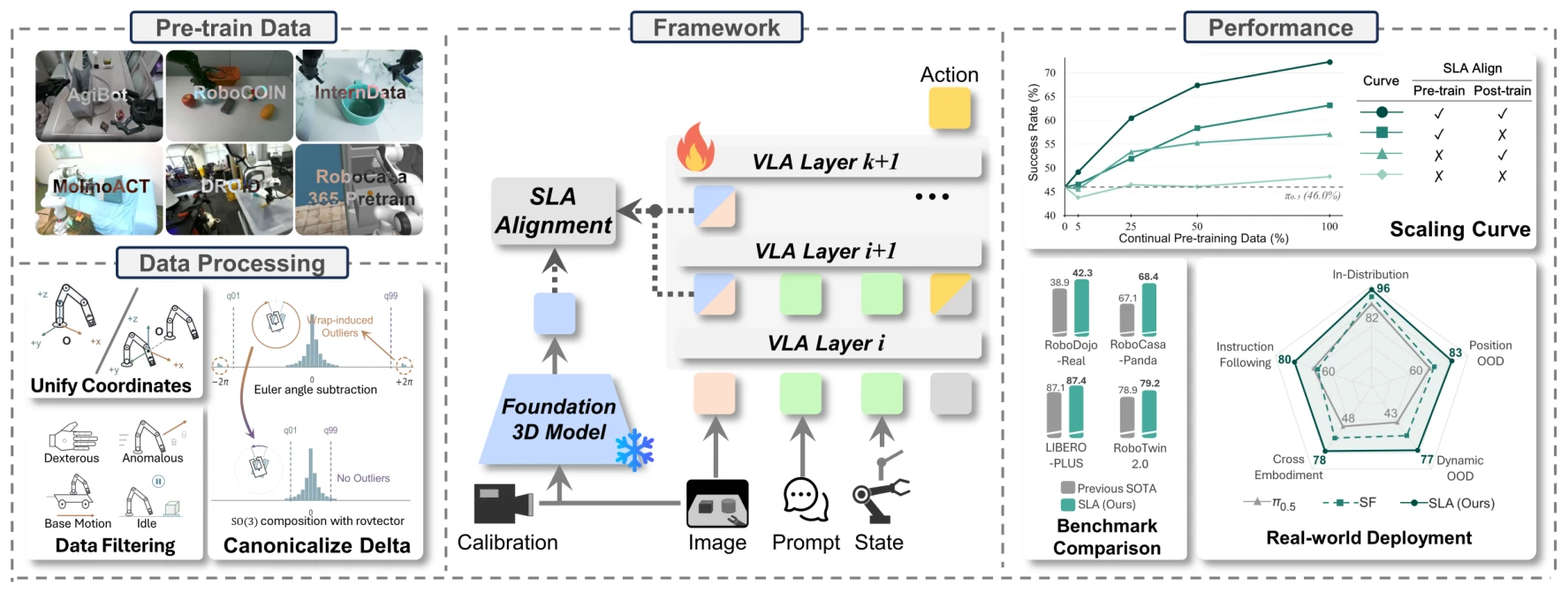
图 1:SLA 统一异构的机器人数据,在训练中把中间层视觉嵌入与冻结的三维特征对齐,并提升了基准测试和真实世界操作的表现。
原图注:SLA unifies heterogeneous robot data, aligns intermediate visual embeddings with frozen 3D features during training, and improves benchmark and real-world manipulation performance.
图 1 解读
图分三栏。左栏“预训练数据”上半是所用数据集的缩略图(AgiBot、RoboCOIN、InternData、MolmoAct、DROID、RoboCasa 预训练集等),下半“数据处理”画了三件事:统一坐标系(Unify Coordinates,把不同机器人的末端坐标系换到同一约定)、数据过滤(Data Filtering,剔除灵巧手、异常、底盘运动、静止片段),以及规范化动作增量(Canonicalize Delta):用欧拉角直接相减会在 \pm\pi 附近产生跨越 2\pi 的离群值(左侧直方图两端的小峰),改用旋转向量并通过 \mathrm{SO}(3) 复合计算相对旋转后离群值消失(右侧直方图)。这一点在第 3.3.2 节和图 3 详述。中栏“框架”:相机标定、图像、文本提示和状态输入 VLA。图像同时送入冻结(雪花图标)的“三维基础模型”,得到空间特征;VLA 第 i、i+1、k+1 等若干层的视觉 token(蓝色方块)被取出,经“SLA 对齐”模块与三维特征对齐。火焰图标表示 VLA 本身是可训练的,最上方输出动作。右栏“性能”:上方“扩展曲线”横轴是持续预训练数据所占比例(0%、5%、25%、50%、100%),纵轴是成功率,四条曲线对应“预训练是否对齐 \times 后训练是否对齐”的四种组合;两阶段都对齐(最深色)最高,到 100% 数据时约 72%,两阶段都不对齐的曲线几乎贴着 \pi_{0.5} 的 46.0% 虚线。左下柱状图把 SLA 与此前最佳结果对比:RoboDojo-Real 42.3 对 38.9,RoboCasa-Panda 68.4 对 67.1,LIBERO-Plus 87.4 对 87.1,RoboTwin 2.0 79.2 对 78.9。右下雷达图是真机部署五个维度:分布内 96、位置 OOD 83、动态 OOD 77、跨本体 78、指令跟随 80;内圈数值(82、60、43、48、60)属于 \pi_{0.5},虚线是 Spatial Forcing(SF)。读这张图时要留意两点:其一,柱状图里有三项领先幅度只有 0.3–1.3 个百分点,属于小幅领先;其二,RoboDojo-Real 的 42.3 是“得分”(Score)而非成功率,正文和摘要中常引用的是成功率 33.9%(见表 5)。
1引言(Introduction)
原文
The development of robotic manipulation hinges on integrating semantic reasoning with accurate physical control in the 3D real world. Recently, vision-language-action (VLA) models (Black et al., 2025; Physical Intelligence, 2025; Yuan et al., 2026a; Team et al., 2026b; Liu et al., 2026b; Bu et al., 2025; Song et al., 2026), capable of instruction following and robotic action execution, have attracted significant attention. By combining the pretrained vision-language model (VLM) with action experts learning on diverse robot demonstrations, these models offer a promising foundation for general-purpose manipulation. However, successful manipulation requires not only recognizing objects and understanding instructions but also executing precise actions in the 3D physical world. Typical 2D VLA foundation models inherit knowledge from VLMs pretrained on 2D image–text pairs and learn robot control without explicitly incorporating 3D physical knowledge during pre-training. This limits their reliability in scenes that demand fine-grained spatial reasoning.
译文
机器人操作的发展取决于能否把语义推理与三维真实世界中的精确物理控制结合起来。近来,能够遵循指令并执行机器人动作的视觉—语言—动作(VLA)模型(Black et al., 2025; Physical Intelligence, 2025; Yuan et al., 2026a; Team et al., 2026b; Liu et al., 2026b; Bu et al., 2025; Song et al., 2026)受到了广泛关注。这些模型把预训练的视觉—语言模型(VLM)与在多样机器人示范上学习的动作专家(action expert)结合起来,为通用操作提供了有前景的基础。然而,成功的操作不仅需要识别物体、理解指令,还需要在三维物理世界中执行精确的动作。典型的二维 VLA 基础模型继承的是在二维图文对上预训练的 VLM 的知识,在预训练期间学习机器人控制时并没有显式融入三维物理知识。这限制了它们在需要细粒度空间推理的场景中的可靠性。
解释
第一段确立“语义”和“空间”两条腿。所谓二维 VLA,是指输入只有 RGB 图像、视觉主干在图文数据上预训练的 VLA,例如 \pi_0、\pi_{0.5};它们并非完全没有空间信息(多视角图像和本体状态里隐含几何),但视觉表征从未被要求编码深度或三维结构。“动作专家”是 \pi_0 系列的术语,指与 VLM 共享注意力、专门用流匹配生成连续动作的那部分 Transformer。
原文
A direct approach to improving spatial understanding is to introduce 3D modalities during post-training on top of a pretrained 2D VLA foundation model. Several approaches (Li et al., 2026a; Sun et al., 2025; Li et al., 2026c) use depth maps or point clouds obtained from depth cameras or other 3D sensors, encode their geometric information, and feed it into the VLM backbone or action head. However, some limitations make it difficult to develop a universal and scalable 3D strategy for this paradigm: (1) Reliable 3D sensor data is hard to acquire, as measured depth maps and point clouds can be noisy or incomplete. (2) Robotic sensors vary in types, positions, and calibration status, which introduces substantial heterogeneity into the data. (3) Portions of existing large-scale robot datasets (O'Neill et al., 2024; Wu et al., 2025b; Lee et al., 2026; Walke et al., 2023; Brohan et al., 2022) do not include depth information, which limits the potential of scaling.
译文
提升空间理解的一种直接做法,是在预训练好的二维 VLA 基础模型之上,于后训练阶段引入三维模态。若干方法(Li et al., 2026a; Sun et al., 2025; Li et al., 2026c)利用深度相机或其他三维传感器得到的深度图或点云,编码其几何信息,再送入 VLM 主干或动作头。然而,一些局限使得这一范式难以发展成通用、可扩展的三维策略:(1) 可靠的三维传感数据难以获取,实测的深度图和点云可能有噪声或不完整;(2) 机器人的传感器在类型、安装位置和标定状态上各不相同,给数据带来很大的异构性;(3) 现有的大规模机器人数据集(O'Neill et al., 2024; Wu et al., 2025b; Lee et al., 2026; Walke et al., 2023; Brohan et al., 2022)中有一部分不含深度信息,这限制了扩展的潜力。
解释
这一段说明为什么不走“显式输入三维”的路。显式方法(如 PointVLA、GeoVLA 一类)推理时也必须有深度或点云输入,于是三个问题一起出现:深度传感器在透明、反光物体上经常给出空洞;不同数据集的相机型号、安装位置、是否标定各不相同;Open X-Embodiment(O'Neill et al.)、Bridge(Walke et al.)、RT-1(Brohan et al.)等大数据集里很多根本没有深度。第三点最致命:如果方法要求深度,就无法用这些数据做大规模预训练。后文的“隐式对齐”正是为绕开这三点而设计的:教师模型只需要 RGB 就能给出三维特征,部署时什么额外输入都不要。
原文
To address these questions, Spatial Forcing (Li et al., 2025a) has propose a implicit 3D representation alignment strategy to enbow 2D VLA with spatial intelligence without explicit demand of depth information. However, Spatial Forcing still concentrate on post-training, leaving spatial competence as a task-specific add-on and limiting the development of scalable 3D VLA foundation models with transferable spatial understanding.
译文
为解决这些问题,Spatial Forcing(Li et al., 2025a)提出了一种隐式三维表征对齐策略,在不显式要求深度信息的情况下赋予二维 VLA 空间智能。然而,Spatial Forcing 仍然只着眼于后训练,使空间能力停留在面向具体任务的附加件上,限制了具有可迁移空间理解能力的可扩展三维 VLA 基础模型的发展。
解释
Spatial Forcing(SF)是同一团队(港科大广州 OpenHelix)此前的工作,也是本文的直接前身:在下游微调时,把 VLA 中间层视觉 token 与冻结的 VGGT 特征做余弦相似度对齐。本文与 SF 的区别可以概括成一句话:SF 只在微调时对齐,SLA 在持续预训练和微调时都对齐,再加上为大规模异构数据配套的若干工程部件。因此 SF 是本文最关键的对照基线(表 11、图 4 都有它)。原文这一段有几处语法错误(has propose、a implicit、enbow 应为 endow、concentrate 应为 concentrates),译文已按原意改正。
原文
Recently, continual pre-training has been widely adopted as a means of developing specific capabilities at scale while preserving the knowledge acquired during foundation model pre-training (Yu et al., 2026; Guo et al., 2026b). Motivated by this approach, we propose to build on the strong 2D foundation model and develop spatial understanding through continual pre-training, laying the foundation for subsequent adaptation. We therefore propose SLA, a robotic foundation model with generalized spatial understanding capabilities developed through implicit representation alignment during both continual pre-training and post-training. Intuitively, action generation is conditioned on visual and linguistic representations, making the spatial content of visual tokens directly relevant to action. Higher-quality visual tokens that contain richer spatial information can facilitate generating more precise manipulation actions. Inspired by this, we align the intermediate visual embeddings of the VLA with external spatial representations extracted from a frozen 3D perception foundation model. This spatial alignment objective complements the standard action-learning objective, encouraging the policy to internalize geometric information in the representations used for action prediction. Crucially, this supervision requires no changes to the pretrained VLA architecture or the action-generation head. We can therefore initialize the policy directly from the pretrained \pi_{0.5} foundation (Physical Intelligence, 2025) and continue training from its learned robotic knowledges. This architectural compatibility allows spatial supervision to shape the foundation model while retaining access to the general knowledge encoded in its pretrained weights.
译文
近来,持续预训练已被广泛用作一种手段:在保留基础模型预训练所得知识的同时,大规模地发展某种特定能力(Yu et al., 2026; Guo et al., 2026b)。受此启发,我们提出在强大的二维基础模型之上,通过持续预训练来发展空间理解,为后续的适配打下基础。为此我们提出 SLA:一个通过在持续预训练和后训练中进行隐式表征对齐而获得泛化空间理解能力的机器人基础模型。直观地看,动作生成以视觉和语言表征为条件,因此视觉 token 中的空间内容与动作直接相关;含有更丰富空间信息的高质量视觉 token 有助于生成更精确的操作动作。受此启发,我们把 VLA 的中间层视觉嵌入与从冻结的三维感知基础模型中提取的外部空间表征对齐。这一空间对齐目标与标准的动作学习目标互为补充,促使策略把几何信息内化到用于动作预测的表征之中。关键在于,这种监督不需要改动预训练 VLA 的架构或动作生成头。因此,我们可以直接用预训练好的 \pi_{0.5} 基础模型(Physical Intelligence, 2025)初始化策略,并在其已学到的机器人知识之上继续训练。这种架构上的兼容性使空间监督能够塑造基础模型,同时保留其预训练权重中编码的通用知识。
解释
“持续预训练”在大语言模型里很常见:拿一个通用模型,在领域数据(代码、数学、医学、金融)上继续以预训练的方式训练,例如 Code Llama、Llemma(参考文献里确实列了 ClinicalBERT、FinBERT、Llemma 等)。本文把这个思路搬到 VLA:不从零训练三维 VLA,而是在 \pi_{0.5} 上继续训练,训练目标从“只预测动作”变成“预测动作 + 视觉表征对齐三维特征”。这一段的论证链条是:动作头通过注意力读取视觉 token \Rightarrow 视觉 token 里空间信息越多,动作越准 \Rightarrow 那就直接监督视觉 token 去编码空间信息。注意这是一个假设性的直觉,作者在第 3.1 节用深度探测实验(图 2)给了一点佐证:冻结 VLA、只训练一个 DPT 深度头时,对齐过的视觉嵌入能解码出更有结构的深度图。但“视觉 token 含更多深度信息”到“动作更准”之间的因果关系,本文主要靠下游成功率的整体提升来间接支持。
原文
Technically, to support continual pre-training across heterogeneous robot data, we combines a unified training corpus. We curate multiple large-scale public datasets covering diverse embodiments, tasks, scenes, and visual appearances, and unify their state and action annotations through consistent end-effector representations and coordinate conventions. This processing provides a common basis for learning how different robots act in space. The resulting visual diversity also makes a single manually chosen alignment layer restrictive: a certain intermediate visual layer of VLA models suited to one domain data may not be equally suitable for another. We therefore develop adaptive layer selection mechanism, using feature-dependent gates to aggregate visual embeddings from multiple VLA layers for spatial supervision. In addition, we adopt OmniVGGT (Peng et al., 2025) as the external 3D perception foundation to exploit partially available camera calibrations and depth annotations alongside RGB images. We further introduce probabilistic state dropout during training to mitigate overfitting to demonstration trajectories and encourage the policy to make better use of visual cues, thereby improving generalization. After continual pre-training, we retain spatial alignment during post-training to adapt the resulting foundation model to specific down-streaming tasks. The teacher, alignment projector, and layer-selection gates are used only during training. At deployment, the policy retains its original inference architecture without requiring the external perception model, alignment projector, or layer-selection gates.
译文
在技术上,为支持在异构机器人数据上进行持续预训练,我们构建了一个统一的训练语料库。我们整理了多个覆盖多样本体、任务、场景和视觉外观的大规模公开数据集,并通过一致的末端执行器表示和坐标约定统一它们的状态与动作标注。这一处理为学习“不同机器人如何在空间中动作”提供了共同的基础。由此带来的视觉多样性也使得手动选定单一对齐层变得受限:适合某一领域数据的 VLA 中间视觉层,未必同样适合另一领域。因此,我们设计了自适应层选择机制,用依赖于特征的门控聚合来自 VLA 多个层的视觉嵌入,用于空间监督。此外,我们采用 OmniVGGT(Peng et al., 2025)作为外部三维感知基础模型,在 RGB 图像之外利用部分可得的相机标定和深度标注。我们还在训练中引入概率性的状态丢弃,以缓解对示范轨迹的过拟合,促使策略更好地利用视觉线索,从而提升泛化能力。持续预训练之后,我们在后训练中保留空间对齐,把得到的基础模型适配到具体的下游任务上。教师模型、对齐投影器和层选择门控只在训练中使用;部署时,策略保持原有的推理架构,不需要外部感知模型、对齐投影器或层选择门控。
解释
这一段是方法部分的提纲,四个部件与摘要第二段一一对应。值得点出它们之间的逻辑关系:数据统一是“能把这么多数据放进一个模型”的前提;数据一多、视觉域一杂,SF 里“手选第几层对齐”的做法就不再合适,于是有了自适应层选择;数据里有的有深度、有的没有,于是选了一个能吃可选几何输入的教师 OmniVGGT(SF 用的是只吃 RGB 的 VGGT);空间监督要起作用,前提是策略真的看图,于是加了状态丢弃,堵住“看状态背轨迹”的捷径。这四件事都只改训练过程,不改推理时的网络。原文 “we combines”“down-streaming” 是笔误。
原文
Extensive evaluations across three public simulation benchmarks, one public real-world benchmark, and eight real-world deployment conditions are conducted to demonstrate the effectiveness of our SLA. On LIBERO-Plus (Fei et al., 2025), it achieves an overall success rate of 87.4% under diverse observation, language, and scene perturbations, outperforming the compared baselines. On RoboTwin 2.0 (Chen et al., 2025a), training on clean demonstrations yields a 72.3% success rate in the Clean2Random setting and a 79.2% average across Clean2Clean and Clean2Random, demonstrating generalization beyond the training conditions. On RoboCasa-Panda (Nasiriany et al., 2024), SLA achieves 68.4% success with only 50 downstream demonstrations per task, exceeding compared policies trained with 300–3,000 demonstrations per task. On RoboDojo-Real (Chen et al., 2026b), a single policy adapted across three embodiments achieves 33.9% overall success, compared with 12.8% for \pi_{0.5}, supporting its applicability to real robot manipulation. Our eight deployment conditions further examine bimanual coordination, spatial and dynamic generalization, few-shot cross-embodiment adaptation, and instruction following. SLA achieves the highest success rate among the compared methods in every condition, averaging 83.8% and improving over \pi_{0.5} by 24.0 percentage points. Controlled data-scaling experiments further show that applying spatial alignment in both training stages outperforms either single-stage alternative at every tested data proportion. Together, these results support developing spatial understanding during continual pre-training and stengthen it during downstream adaptation.
译文
我们在三个公开仿真基准、一个公开真实世界基准和八种真实世界部署条件上进行了大量评估,以证明 SLA 的有效性。在 LIBERO-Plus(Fei et al., 2025)上,它在多种观测、语言和场景扰动下取得 87.4% 的总体成功率,超过了所比较的基线。在 RoboTwin 2.0(Chen et al., 2025a)上,用干净示范训练,在 Clean2Random 设定下取得 72.3% 的成功率,在 Clean2Clean 与 Clean2Random 上的平均为 79.2%,表明其能泛化到训练条件之外。在 RoboCasa-Panda(Nasiriany et al., 2024)上,SLA 每个任务只用 50 条下游示范就取得 68.4% 的成功率,超过了每任务使用 300–3,000 条示范训练的对比策略。在 RoboDojo-Real(Chen et al., 2026b)上,一个在三种本体上适配的单一策略取得 33.9% 的总体成功率,而 \pi_{0.5} 为 12.8%,支持了它在真实机器人操作中的适用性。我们的八种部署条件进一步考察了双臂协调、空间与动态泛化、少样本跨本体适配以及指令跟随。SLA 在每一种条件下都取得了所比较方法中最高的成功率,平均为 83.8%,比 \pi_{0.5} 高 24.0 个百分点。受控的数据扩展实验还表明,在两个训练阶段都施加空间对齐,在每一个测试的数据比例下都优于只在单一阶段对齐的两种做法。这些结果共同支持:在持续预训练中发展空间理解,并在下游适配中加以强化。
解释
几个数字可以先验算一下。RoboTwin 2.0:72.3% 是 Clean2Random,平均 79.2% 意味着 Clean2Clean 约为 2\times79.2-72.3=86.1\%(表 3 中为 86.0,平均 79.15 四舍五入为 79.2)。RoboDojo-Real 的 33.9% 是三种本体成功率的等权平均 (36.7+55.0+10.0)/3=33.9,\pi_{0.5} 为 (13.3+21.7+3.3)/3=12.8,相对提升约 2.6 倍;但在同一张表里,InternW0-\Delta 的成功率是 31.7%,SLA 只领先 2.2 个百分点,引言没有提这一点。八种部署条件的平均 83.8% 与 \pi_{0.5} 的 59.8% 都能由表 11 逐项相加除以 8 精确还原(670/8=83.75,478/8=59.75),差正好 24.0。RoboCasa-Panda 的“50 条对 300–3,000 条”要看清口径:对比方法用多少示范来自各自论文的设置,SLA 自己则经过了包含 RoboCasa365 预训练子集的持续预训练(作者称已排除下游评测数据,但场景和资产属于同一仿真平台)。因此这一比较说明的是“预训练 + 少量下游示范”的整体效率,不能单纯归功于空间对齐。原文 “stengthen” 为笔误。
原文
Our contributions are summarized as follows:
- We introduce SLA, a robotic foundation model that implicitly enforces the integration of visual embeddings in VLAs with external spatial representations.
- We extend SLA to continual pre-training on a carefully curated and unified corpus of public robot datasets, developing a spatially informed foundation model.
- We apply SLA training principle during downstream post-training and demonstrate strong benchmark performance, together with bimanual coordination, spatial and dynamic generalization, few-shot cross-embodiment adaptation, and instruction following.
译文
我们的贡献总结如下:
- 我们提出 SLA,一个机器人基础模型,它隐式地促使 VLA 中的视觉嵌入与外部空间表征相融合。
- 我们把 SLA 扩展到持续预训练,在一个精心整理并统一的公开机器人数据语料库上训练,得到一个具备空间信息的基础模型。
- 我们在下游后训练中沿用 SLA 的训练原则,展示了强劲的基准性能,以及双臂协调、空间与动态泛化、少样本跨本体适配和指令跟随能力。
解释
三条贡献分别对应“对齐方法”“持续预训练”“下游效果”。坦白说,第一条的核心机制(中间层视觉 token 与冻结三维模型特征做余弦对齐)在 Spatial Forcing 中已经提出,本文在方法层面的新增主要是把它搬到持续预训练阶段以及配套的门控多层聚合、OmniVGGT 教师、状态丢弃和数据统一流程。读后文实验时,最能检验本文主张的是表 6/图 4 的“预训练对齐 \times 后训练对齐”消融,以及表 11 中 SLA 与 SF 的直接对比。
2相关工作(Related Work)
2.1VLA 基础模型(VLA Foundation Models)
原文
VLA foundation models learn generalist manipulation policies from large, diverse datasets and adapt them to downstream tasks. Cross-embodiment datasets (O'Neill et al., 2024; Walke et al., 2023; Brohan et al., 2022; Wu et al., 2024; Fang et al., 2024; Allshire et al., 2026; Jiang et al., 2026) have accelerated this development. OpenVLA (Kim et al., 2024), \pi_0 (Black et al., 2025), RDT-1B (Liu et al., 2024), and GR00T N1 (Bjorck et al., 2025) learn language-conditioned action prediction from robot demonstrations, while GR-2 (Cheang et al., 2024) combines large-scale video pre-training with policy learning on robot trajectories. To improve task understanding, RT-H (Belkhale et al., 2024) and \pi_{0.5} (Physical Intelligence, 2025) adopt language-conditioned task hierarchies, whereas MolmoAct (Lee et al., 2026) and MolmoAct2 (Fang et al., 2026) incorporate action reasoning into robot control. RT-2 (Brohan et al., 2023), \pi_{0.5}, and Xiaomi-Robotics-0 (Cai et al., 2026b) also co-train on robot and vision-language data to support semantic generalization and instruction following.
译文
VLA 基础模型从大规模、多样化的数据集中学习通用操作策略,并适配到下游任务。跨本体数据集(O'Neill et al., 2024; Walke et al., 2023; Brohan et al., 2022; Wu et al., 2024; Fang et al., 2024; Allshire et al., 2026; Jiang et al., 2026)加速了这一发展。OpenVLA(Kim et al., 2024)、\pi_0(Black et al., 2025)、RDT-1B(Liu et al., 2024)和 GR00T N1(Bjorck et al., 2025)从机器人示范中学习以语言为条件的动作预测,而 GR-2(Cheang et al., 2024)把大规模视频预训练与在机器人轨迹上的策略学习结合起来。为改进任务理解,RT-H(Belkhale et al., 2024)和 \pi_{0.5}(Physical Intelligence, 2025)采用以语言为条件的任务层级,而 MolmoAct(Lee et al., 2026)和 MolmoAct2(Fang et al., 2026)则把动作推理融入机器人控制。RT-2(Brohan et al., 2023)、\pi_{0.5} 和 Xiaomi-Robotics-0(Cai et al., 2026b)还在机器人数据和视觉—语言数据上联合训练,以支持语义泛化和指令跟随。
解释
这一段按“做了什么改进”给 VLA 分类:纯动作预测(OpenVLA、\pi_0、RDT、GR00T)、引入视频预训练(GR-2)、引入任务层级或推理(RT-H、\pi_{0.5} 的高层子任务预测,MolmoAct 的“动作推理链”),以及与网络图文数据联合训练(RT-2、\pi_{0.5})。这些改进都集中在语义一侧;下一段才引出本文关心的“空间”一侧。MolmoAct 的数据后来也被本文用作持续预训练语料的一部分(表 1)。
原文
The scarcity of teleoperated robot data has further motivated alternative sources of supervision. HumanScale (Ma et al., 2026) investigates pre-training on egocentric human videos followed by adaptation with robot data. Separately, the Universal Manipulation Interface (UMI) (Chi et al., 2024) enables portable demonstration collection using handheld grippers without requiring robots at collection sites. RDT2 (Liu et al., 2026a) and Xiaomi-Robotics-1 (Team et al., 2026b) exploit UMI data to expand training scale and coverage of environments and tasks. These advances support generalist action learning, but data scaling alone does not specify how geometric representations should be supervised during pre-training. Our complementary goal is to develop 3D spatial understanding in an existing VLA foundation model through spatially supervised continual pre-training.
译文
遥操作机器人数据的稀缺还促使人们寻找其他监督来源。HumanScale(Ma et al., 2026)研究了先在第一人称人类视频上预训练、再用机器人数据适配的方案。另一方面,通用操作接口(Universal Manipulation Interface,UMI)(Chi et al., 2024)借助手持夹爪实现便携式示范采集,采集现场不需要机器人。RDT2(Liu et al., 2026a)和 Xiaomi-Robotics-1(Team et al., 2026b)利用 UMI 数据扩大训练规模,以及环境和任务的覆盖面。这些进展支持了通用动作学习,但仅仅扩大数据规模并没有说明在预训练中应如何监督几何表征。我们的目标与之互补:通过带空间监督的持续预训练,在已有的 VLA 基础模型中发展三维空间理解。
解释
这一段收束于本文定位:别人在解决“数据从哪来”,本文解决“数据来了以后,视觉表征该往什么方向学”。换言之,本文的贡献与扩数据并不冲突,空间对齐损失原则上可以叠加在任何一种扩数据方案上。本文自己的持续预训练语料(约 1.7M 回合,表 1)全部来自公开的机器人数据,没有使用人类视频或 UMI 数据。
2.2三维 VLA 模型(3D VLA Models)
原文
Existing 3D VLA methods introduce geometry through explicit inputs, feature fusion, or representation supervision. PointVLA (Li et al., 2026a) and GeoVLA (Sun et al., 2025) integrate point cloud features into action prediction. BridgeVLA (Li et al., 2026c) projects 3D observations into multi-view images; and FALCON (Zhang et al., 2025) extracts geometric tokens from spatial foundation models for fusion within the action head. These approaches still require additional geometric input extraction at deployment. Another works use training-time supervision to encode spatial structure in internal policy representations. ROCKET (Sun et al., 2026) explores multilayer spatial alignment, VEGA (Wang et al., 2026a) supervises visual encoder outputs, and Mind-VLA (Ding et al., 2026) introduces instruction-aware alignment of target-object representations.
译文
现有的三维 VLA 方法通过显式输入、特征融合或表征监督引入几何信息。PointVLA(Li et al., 2026a)和 GeoVLA(Sun et al., 2025)把点云特征融入动作预测。BridgeVLA(Li et al., 2026c)把三维观测投影为多视角图像;FALCON(Zhang et al., 2025)则从空间基础模型中提取几何 token,在动作头内部融合。这些方法在部署时仍然需要额外提取几何输入。另一些工作利用训练时的监督,把空间结构编码进策略的内部表征:ROCKET(Sun et al., 2026)探索多层空间对齐,VEGA(Wang et al., 2026a)监督视觉编码器的输出,Mind-VLA(Ding et al., 2026)引入对目标物体表征的、感知指令的对齐。
解释
三维 VLA 的两条路线在这里划得很清楚。显式路线(PointVLA、GeoVLA、BridgeVLA、FALCON)把点云、深度或三维基础模型的特征当作额外输入,推理时也要算;隐式路线(Spatial Forcing、ROCKET、VEGA、Mind-VLA)只在训练时加监督,推理时网络不变。本文属于隐式路线,而且和 ROCKET 一样做多层对齐,区别在于本文的多层权重由依赖于特征的门控逐 token、逐通道决定(第 3.2.3 节)。FALCON 介于两者之间:它也用空间基础模型,但把几何 token 作为输入融进动作头,推理时必须保留。
原文
Such approaches emphasize adding 3D capabilities during post-training on top of generic 2D VLA pre-training (Physical Intelligence, 2025; Bu et al., 2025; Kim et al., 2025), leaving spatial understanding as a supplementary capability rather than establishing a scalable 3D-aware foundation. Recent studies incorporate geometry into pre-training through egocentric spatial embeddings (Qu et al., 2025), egocentric 3D annotations (Feng et al., 2026), and object pose estimation (Lin et al., 2026). However, these 3D-aware pre-training efforts remain relatively limited in scale compared with large-scale 2D VLA pre-training. In contrast, we build on pretrained 2D VLA through continual pre-training to develop generalizable 3D-aware foundation models.
译文
这些方法着重于在通用二维 VLA 预训练(Physical Intelligence, 2025; Bu et al., 2025; Kim et al., 2025)之上,于后训练阶段添加三维能力,使空间理解成为一种补充能力,而没有建立可扩展的、具备三维感知的基础模型。近期一些研究通过以自我为中心的空间嵌入(Qu et al., 2025)、第一人称三维标注(Feng et al., 2026)和物体位姿估计(Lin et al., 2026)把几何信息引入预训练。然而,与大规模二维 VLA 预训练相比,这些三维感知预训练工作的规模仍相对有限。与之不同,我们在预训练好的二维 VLA 之上通过持续预训练,发展具有泛化能力的三维感知基础模型。
解释
这里给出本文相对两类工作的定位:相对“后训练加三维”的方法,本文把三维监督提前到预训练;相对“从头做三维预训练”的方法(如 SpatialVLA,即 Qu et al., 2025,它在预训练中引入 Ego3D 位置编码,需要深度估计),本文不从头训练,而是站在 \pi_{0.5} 的肩膀上继续训练,因此能直接继承二维预训练的规模优势。SpatialVLA 也出现在表 11 的真机对比里。
2.3持续预训练(Continual Pre-training)
原文
Continual pre-training extends the domain capabilities of existing foundation models through further large-scale pre-training, providing a basis for downstream adaptation. Early studies (Lee et al., 2020; Alsentzer et al., 2019; Araci, 2019; Chalkidis et al., 2020; Gururangan et al., 2020) focus on adapting to domain-specific data distributions. Llemma (Azerbayev et al., 2024) strengthens mathematical reasoning through continual pre-training on mathematical text and code. AgentFounder (Su et al., 2026b) uses diverse reasoning and action data to establish a foundation for agent capabilities before post-training. Recent efforts extend this paradigm to robotics: ET-VLA (Li and Peng, 2025) uses synthetic data for continual pre-training to transfer existing VLAs to new embodiments, whereas AXIS (Zhao et al., 2026) investigates how policy performance scales with data. These VLA efforts primarily focus on training data sources. In contrast, we use implicit spatial alignment framework during continual pre-training to develop generalizable 3D spatial understanding while preserving the pretrained VLA backbone architecture.
译文
持续预训练通过进一步的大规模预训练来扩展已有基础模型在特定领域的能力,为下游适配提供基础。早期研究(Lee et al., 2020; Alsentzer et al., 2019; Araci, 2019; Chalkidis et al., 2020; Gururangan et al., 2020)着重于适配特定领域的数据分布。Llemma(Azerbayev et al., 2024)通过在数学文本和代码上持续预训练来增强数学推理。AgentFounder(Su et al., 2026b)在后训练之前用多样的推理和行动数据为智能体能力打下基础。近期的工作把这一范式扩展到机器人领域:ET-VLA(Li and Peng, 2025)用合成数据做持续预训练,把已有的 VLA 迁移到新本体上;AXIS(Zhao et al., 2026)则研究策略性能如何随数据扩展。这些 VLA 工作主要关注训练数据的来源。与之不同,我们在持续预训练中使用隐式空间对齐框架,在保持预训练 VLA 主干架构的同时,发展具有泛化能力的三维空间理解。
解释
早期引用依次是 BioBERT(生物医学)、ClinicalBERT(临床)、FinBERT(金融)、LEGAL-BERT(法律)以及 Gururangan 等人的“Don't Stop Pretraining”,后者系统说明了“领域自适应预训练”和“任务自适应预训练”都能提升下游效果。本文与机器人领域已有持续预训练工作(ET-VLA、AXIS)的区别是:它们改变的是数据,本文还改变了目标函数(加入空间对齐损失)。这一区分也决定了本文最需要回答的问题:在同样的持续预训练数据上,加不加对齐损失有多大差别?这正是第 4.4.1 节数据扩展消融要回答的。
3方法(Methodology)
原文
SLA aims to develop a scalable 3D VLA foundation model through continual pre-training. Starting from a pretrained 2D VLA backbone (Physical Intelligence, 2025), we use external spatial representation supervision to shape its visual representations while retaining its backbone and action-generation architecture. Sec. 3.1 motivates this approach, Sec. 3.2 presents the model and training mechanisms, and Sec. 3.3 describes the continual-pre-training corpus and its unified processing.
译文
SLA 的目标是通过持续预训练发展一个可扩展的三维 VLA 基础模型。我们从一个预训练好的二维 VLA 主干(Physical Intelligence, 2025)出发,用外部空间表征作为监督来塑造它的视觉表征,同时保留其主干和动作生成架构。第 3.1 节说明这一做法的动机,第 3.2 节介绍模型和训练机制,第 3.3 节介绍持续预训练语料库及其统一处理流程。
解释
本节的结构:3.1 先用“深度探测”实验说明二维 VLA 的视觉嵌入缺空间信息;3.2 给出对齐损失(式 3–6)、教师模型、门控层选择(式 7)和状态丢弃;3.3 讲数据,包括坐标统一和旋转表示(式 8–10)。
3.1动机(Motivation)
原文
VLA models are built upon pretrained VLMs and generate actions through specialized designs for action experts. A \theta-parameterized VLM model employs multiple causal attention layers in an auto-regressive manner to generate the next tokens, formed as \bm{x}_t \sim p_\theta(\bm{x}_t \mid \bm{x}_{<t}), where \{\bm{x}_t\}_{t=1}^T denotes a sequence of tokens.
译文
VLA 模型建立在预训练的 VLM 之上,并通过为动作专家专门设计的结构来生成动作。一个以 \theta 为参数的 VLM 使用多个因果注意力层,以自回归的方式生成下一个 token,形式为 \bm{x}_t \sim p_\theta(\bm{x}_t \mid \bm{x}_{<t}),其中 \{\bm{x}_t\}_{t=1}^T 表示一个 token 序列。
解释
这是标准的语言模型写法:第 t 个 token 的分布只依赖于它之前的 token(“因果”指注意力只能看前面)。下一段把序列拆成视觉、语言、动作三段。
原文
When adapted to VLA models, three modalities of information will be processed: vision, text, and action. The vision modality consists of multi-view images captured by robots, which are transformed into N visual tokens \{\bm{x}_t^\mathcal{V}\}_{t=1}^N through pretrained visual encoders such as DINOv2 (Oquab et al., 2023) or SigLIP (Zhai et al., 2023). The text modality consists of task instructions, which are converted into M linguistic tokens \{\bm{x}_t^\mathcal{L}\}_{t=1}^M by a text tokenizer. Then, the VLA models generate K action tokens \{\bm{x}_t^\mathcal{A}\}_{t=1}^K conditioned on the preceding visual and linguistic tokens:
\bm{x}_t^\mathcal{A} \sim p_\theta \big(\bm{x}_t^\mathcal{A} \mid \{\bm{x}_i^\mathcal{V}\}_{i=1}^N, \{\bm{x}_j^\mathcal{L}\}_{j=1}^M, \bm{x}_{<t}^\mathcal{A} \big),(1)
\mathcal{L}_{\mathrm{action}} = \mathcal{L}[\mathcal{G}(\{\bm{x}_t^\mathcal{A}\}_{t=1}^K), A_{gt}],(2)
where \mathcal{L}[\cdot,\cdot] denotes the training loss (e.g. L1, L2, or cross-entropy loss), \mathcal{G} denotes the trainable action expert (e.g. multi-layer MLP or flow-matching head (Lipman et al., 2022)). Eq. (1) illustrates that the visual tokens as intermediate scene representations play a crucial role in generating action tokens and should be supervised properly. 译文
用于 VLA 模型时,需要处理三种模态的信息:视觉、文本和动作。视觉模态由机器人拍摄的多视角图像组成,经 DINOv2(Oquab et al., 2023)或 SigLIP(Zhai et al., 2023)等预训练视觉编码器转换为 N 个视觉 token \{\bm{x}_t^\mathcal{V}\}_{t=1}^N。文本模态由任务指令组成,经文本分词器转换为 M 个语言 token \{\bm{x}_t^\mathcal{L}\}_{t=1}^M。随后,VLA 模型以前面的视觉和语言 token 为条件,生成 K 个动作 token \{\bm{x}_t^\mathcal{A}\}_{t=1}^K:
\bm{x}_t^\mathcal{A} \sim p_\theta \big(\bm{x}_t^\mathcal{A} \mid \{\bm{x}_i^\mathcal{V}\}_{i=1}^N, \{\bm{x}_j^\mathcal{L}\}_{j=1}^M, \bm{x}_{<t}^\mathcal{A} \big),(1)
\mathcal{L}_{\mathrm{action}} = \mathcal{L}[\mathcal{G}(\{\bm{x}_t^\mathcal{A}\}_{t=1}^K), A_{gt}],(2)
其中 \mathcal{L}[\cdot,\cdot] 表示训练损失(如 L1、L2 或交叉熵损失),\mathcal{G} 表示可训练的动作专家(如多层 MLP 或流匹配头(Lipman et al., 2022))。式 (1) 表明,视觉 token 作为中间的场景表征,在生成动作 token 时起着关键作用,应当受到恰当的监督。 解释
符号:上标 \mathcal V、\mathcal L、\mathcal A 分别标记视觉、语言、动作 token;N 是所有视角的视觉 token 总数(\pi_{0.5} 的 SigLIP 对每张 224\times224 图像给出 16\times16=256 个 token,三路相机就是 768 个);A_{gt} 是示范中的真值动作;\mathcal G 把动作 token 解码为连续动作。式 (1) 是一个通用的写法,同时覆盖离散动作 token 的 OpenVLA(交叉熵)和连续动作的 \pi_0 类模型(流匹配)。对 \pi_{0.5} 而言,“动作 token”实际上是动作专家中对应带噪动作的那些位置,\mathcal L 是流匹配的速度回归损失。论证的要点在最后一句:式 (1) 中动作只能“通过视觉 token 看到场景”,所以视觉 token 的质量是动作质量的上限之一。然而标准训练只用式 (2) 这一个动作损失,视觉 token 只能从动作误差反传回来的间接信号中学习空间结构。本文的做法就是给视觉 token 加一个直接的监督信号。
原文
Since VLA models must capture 3D information and reason about the relative positions between robots and objects to generate precise spatial movements, we hypothesize that the 3D information is implicitly embedded within the visual embeddings of VLAs. Such embeddings would allow action tokens to acquire 3D cues through the auto-regressive mechanism during inference.
译文
由于 VLA 模型必须捕捉三维信息、推理机器人与物体之间的相对位置,才能生成精确的空间运动,我们假设三维信息隐式地嵌入在 VLA 的视觉嵌入之中。这样的嵌入会让动作 token 在推理时通过自回归机制获得三维线索。
解释
这是一个待检验的假设:如果 VLA 真的能做精确操作,它的视觉嵌入里“应该”已经有三维信息。下一段的探测实验给出的答案是否定的:未经对齐的嵌入里,能解码出的深度结构很差。这一“假设—否定”的结构是为了引出“需要显式监督视觉嵌入”。
原文
To evaluate this hypothesis, we follow linear probing (He et al., 2020; Wu et al., 2025a) to conduct a lightweight depth probing experiment. Specifically, we freeze all the parameters of a VLA model (Kim et al., 2025) and only train a DPT head (Ranftl et al., 2021) to transform the visual embeddings of VLA to depth maps. This enables us to quantify the richness of spatial information embedded in the VLA representation space. As shown in Fig. 2, the probing results show that visual embeddings learned solely from 2D images do not produce meaningful spatial structures, suggesting a limited capacity of the model to encode 3D structure information without explicit spatial input or guidance.
译文
为检验这一假设,我们仿照线性探测(linear probing)(He et al., 2020; Wu et al., 2025a)的做法,进行了一个轻量的深度探测实验。具体而言,我们冻结一个 VLA 模型(Kim et al., 2025)的全部参数,只训练一个 DPT 头(Ranftl et al., 2021),把 VLA 的视觉嵌入转换为深度图。这使我们能够量化 VLA 表征空间中所蕴含空间信息的丰富程度。如图 2 所示,探测结果表明,仅从二维图像中学到的视觉嵌入无法生成有意义的空间结构,说明在没有显式空间输入或引导的情况下,模型编码三维结构信息的能力有限。
解释
探测(probing)是表征学习里的常用诊断:冻结被测模型,只在其特征上训练一个小读出头,读出头越容易学好,说明特征里越“现成地”包含这种信息。经典做法是线性分类器(He et al. 的 MoCo);这里用的是 DPT 头(Dense Prediction Transformer 的解码头,含卷积和多尺度融合),比线性层强得多,因此严格说并非“线性探测”,只是借用了其思路。需要注意三点口径。第一,被探测的 VLA 是 OpenVLA-OFT(Kim et al., 2025),而不是 SLA 所基于的 \pi_{0.5};“对齐后”的嵌入应来自 Spatial Forcing 式的对齐训练,正文没有交代具体是哪个模型、在什么数据上对齐。第二,正文说“量化”空间信息的丰富程度,但图 2 只给了定性的深度图,没有给出深度误差等数值指标。第三,探测头能读出深度说明特征里有深度信息,但这并不直接证明动作因此更准;后者要靠第 4 节的下游实验。
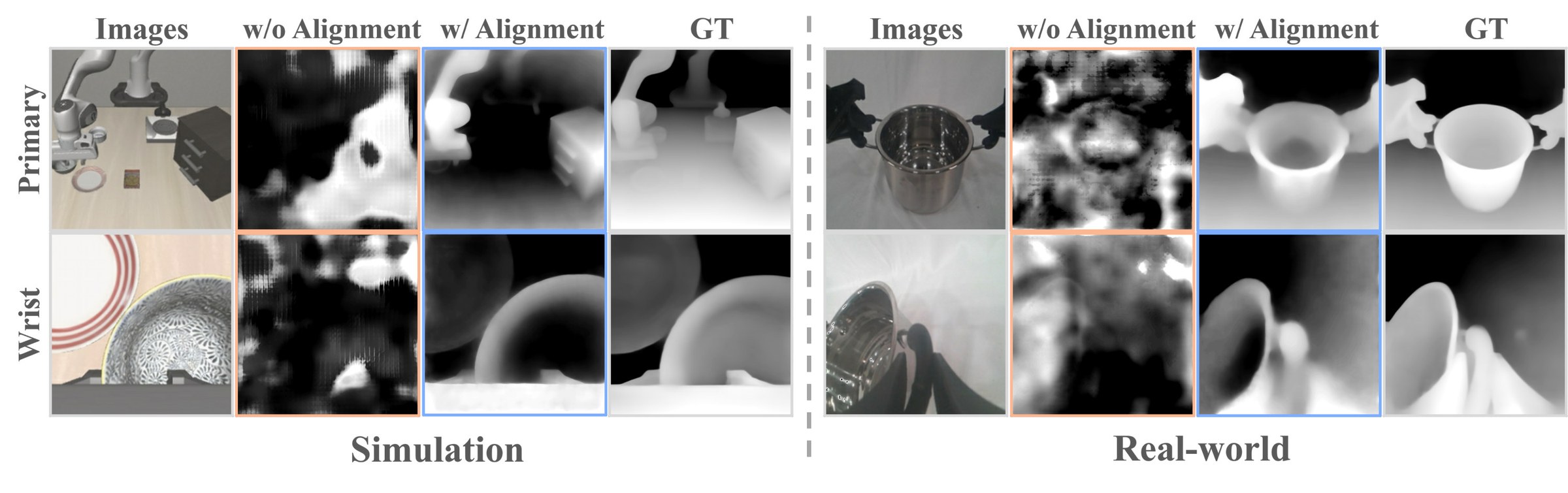
图 2:VLA 视觉嵌入的深度探测。仅从二维图像学习、未经对齐的嵌入无法生成有意义的空间结构。对齐后的嵌入本身就包含丰富的空间信息,因而在深度探测中表现更好。
原图注:Depth probing of the visual embeddings of VLAs. Embeddings learned solely from 2D images without alignment do not produce meaningful spatial structures. The aligned embeddings inherently contain rich spatial information, leading to better performance in depth probing.
图 2 解读
左半是仿真(LIBERO 风格的厨房桌面),右半是真机(双臂抓着一个不锈钢锅)。每半边上一行是主视角(Primary)相机,下一行是腕部(Wrist)相机。四列依次是:输入图像;未对齐的 VLA 嵌入经 DPT 头解码出的深度(橙框);对齐后的嵌入解码出的深度(蓝框);真值深度(GT)。深度图中越亮表示越近。“未对齐”一列基本是斑块状的噪声,只隐约看得出大块明暗,物体轮廓几乎不可辨;“对齐后”一列能清楚还原机械臂、抽屉柜、盘子边缘、锅的形状,与 GT 十分接近,尤其是右侧真机的锅(不锈钢强反光,正是深度传感器容易出空洞的情形)。这张图是定性展示,只给了 4 组样例,没有统计意义上的指标;它的作用是让读者直观接受“二维预训练的视觉 token 里缺乏可读出的几何结构,而对齐可以补上”这一前提。
原文
However, bridging this 3D physical gap through additional sensor inputs or depth-estimation modules would change the architecture of the original 2D VLA foundation model and may disrupt the general knowledge already acquired during its pre-training. We therefore seek a training strategy that reuses the existing VLA architecture and pretrained parameters to unlock its generalizable understanding of the 3D physical world through continual pre-training.
译文
然而,通过额外的传感器输入或深度估计模块来弥合这一三维物理鸿沟,会改变原有二维 VLA 基础模型的架构,并可能破坏它在预训练中已经获得的通用知识。因此,我们寻求一种训练策略:复用已有的 VLA 架构和预训练参数,通过持续预训练释放其对三维物理世界的可泛化理解。
解释
这里给出了“不改架构”的第二个理由(第一个是引言里说的部署时不需要深度传感器):新加的输入分支是随机初始化的,会扰动已经训好的注意力分布,模型需要大量数据重新适应,而预训练知识可能在这一过程中被冲掉。只加一个辅助损失,则所有原有参数都从预训练值出发、只是被额外的梯度推一推。当然,辅助损失同样会改变视觉 token,是否损害语义能力(如指令跟随)需要实验检验;表 2 中 SLA 在 LIBERO-Plus 的 Language 维度(83.5)低于 SF(85.6),可算作一个值得留意的信号。
3.2模型(Model)
3.2.1模型架构(Model Architecture)
原文
Our main philosophy is to employ external supervision signals to supervise the visual tokens \bm{x}^{\mathcal V}. To provide the signals with rich spatial information, we first input a set of multi-view images \mathcal I into a frozen external 3D perception foundation model f^{\mathrm{3D}}, which outputs pixel-level 3D representations f^{\mathrm{3D}}(\mathcal I) for each image. Available geometric annotations like camera parameters and depth images are also provided to this external 3D foundation model, as described in Sec. 3.2.2. Additionally, these spatial representations are augmented with positional embeddings E to ensure that the supervised tokens preserve the critical spatial position order during supervised training. We extract the final-layer representations of f^{\mathrm{3D}}(\mathcal I) and bilinearly resample the feature grids with positional embeddings to the VLA token resolution, obtaining a spatial target \mathbf y_i at each visual token location:
\mathbf y=\mathcal R\!\left[f^{\mathrm{3D}}(\mathcal I)+E\right],(3)
where \mathcal R\left[\cdot\right] denotes bilinear resampling to the VLA visual token resolution. For brevity, the available geometric annotations like camera parameters are implicit in \mathcal I. 译文
我们的核心思路是用外部监督信号来监督视觉 token \bm{x}^{\mathcal V}。为了让这一信号带有丰富的空间信息,我们先把一组多视角图像 \mathcal I 输入一个冻结的外部三维感知基础模型 f^{\mathrm{3D}},它为每幅图像输出像素级的三维表征 f^{\mathrm{3D}}(\mathcal I)。如第 3.2.2 节所述,相机参数、深度图等可得的几何标注也一并提供给这个外部三维基础模型。此外,这些空间表征还叠加了位置嵌入 E,以确保被监督的 token 在监督训练中保持关键的空间位置顺序。我们提取 f^{\mathrm{3D}}(\mathcal I) 的最后一层表征,把叠加了位置嵌入的特征网格双线性重采样到 VLA 的 token 分辨率,在每个视觉 token 的位置上得到空间目标 \mathbf y_i:
\mathbf y=\mathcal R\!\left[f^{\mathrm{3D}}(\mathcal I)+E\right],(3)
其中 \mathcal R\left[\cdot\right] 表示双线性重采样到 VLA 视觉 token 的分辨率。为简洁起见,相机参数等可得的几何标注隐含在 \mathcal I 中。 解释
式 (3) 构造的是对齐目标。三步:(1) 冻结的教师 f^{\mathrm{3D}}(OmniVGGT)对多视角图像做一次前向,取最后一层的逐 patch 特征;(2) 加上位置嵌入 E;(3) 用双线性插值把教师的特征网格缩放到 VLA 的 token 网格(例如 16\times16),使教师特征与 VLA 视觉 token 一一对应。为什么要加位置嵌入?余弦对齐是逐 token 进行的,如果目标里只有“语义—几何内容”,两个外观相似但位置不同的 patch 目标几乎一样;叠加 E 后,目标向量还携带“我在图像的哪个位置”,迫使 VLA 的 token 保留空间排布信息。这一设计沿用自 Spatial Forcing。正文没有说明 E 是固定的正弦编码还是可学习的,也没有给出教师特征的维度。
原文
To align the VLA's per-pixel visual tokens with this external 3D perception foundation model, we first process each VLA visual token \bm{x}^{\mathcal V} with layer normalization \mathrm{LN} followed by a two-layer MLP to ensure compatibility in feature dimension. Let {}^{(\ell)}\bm{x}^{\mathcal V} denote the VLA visual tokens after attention layer \ell of the VLA's vision-language backbone. The normalization and MLP parameters are shared across layers. As there are multiple causal attention layers in the VLA model, visual tokens can be obtained after different layers. We adaptively aggregate their projected features into \mathbf z:
\begin{aligned} \mathbf z &=\mathcal F\!\left[\left\{{}^{(\ell)}\bm{x}^{\mathcal V}\right\}_{\ell=1}^{L}\right] =\sum_{\ell=1}^{L}{}^{(\ell)}\mathbf g\odot \mathrm{MLP}\!\left[\mathrm{LN}\!\left({}^{(\ell)}\bm{x}^{\mathcal V}\right)\right], \end{aligned}(4)
where L is the number of VLA attention layers, {}^{(\ell)}\mathbf g_i is a token- and channel-wise gate, and \odot denotes element-wise multiplication. This fusion operator \mathcal F\left[\cdot\right] denotes the adaptive layer selection strategy, which is detailed in Sec. 3.2.3. 译文
为了把 VLA 的逐像素视觉 token 与这个外部三维感知基础模型对齐,我们先对每个 VLA 视觉 token \bm{x}^{\mathcal V} 做层归一化 \mathrm{LN},再接一个两层 MLP,以保证特征维度匹配。记 {}^{(\ell)}\bm{x}^{\mathcal V} 为 VLA 视觉—语言主干第 \ell 个注意力层之后的视觉 token。归一化和 MLP 的参数在各层之间共享。由于 VLA 模型中有多个因果注意力层,可以在不同层之后取得视觉 token。我们把它们投影后的特征自适应地聚合为 \mathbf z:
\begin{aligned} \mathbf z &=\mathcal F\!\left[\left\{{}^{(\ell)}\bm{x}^{\mathcal V}\right\}_{\ell=1}^{L}\right] =\sum_{\ell=1}^{L}{}^{(\ell)}\mathbf g\odot \mathrm{MLP}\!\left[\mathrm{LN}\!\left({}^{(\ell)}\bm{x}^{\mathcal V}\right)\right], \end{aligned}(4)
其中 L 是 VLA 注意力层的数量,{}^{(\ell)}\mathbf g_i 是逐 token、逐通道的门控,\odot 表示逐元素相乘。这个融合算子 \mathcal F\left[\cdot\right] 就是自适应层选择策略,详见第 3.2.3 节。 解释
式 (4) 构造的是对齐的“学生”一侧。每一层 \ell 的视觉 token 先经过同一个 \mathrm{LN}+两层 MLP 投影到教师特征的维度,再乘以门控 {}^{(\ell)}\mathbf g(与投影后特征同维、取值在 (0,1)),最后对 L 层求和。对 \pi_{0.5} 来说,视觉—语言主干是 Gemma 2B,有 18 层,所以 L=18,每个视觉 token 位置都要汇总 18 层的信息。与 Spatial Forcing 的区别在这里:SF 只取某一个手选的层做对齐,SLA 让所有层都参与、由门控决定各层的权重(第 4.4.2 节表 7 比较了固定取第 1、6、12、18 层与自适应融合)。这样做的副作用是,对齐损失的梯度会流入所有层,而不只是某一层之前的部分。原文排版中式 (4) 的门控写作 {}^{(\ell)}\mathbf g(无下标),随后解释为 {}^{(\ell)}\mathbf g_i(带 token 下标 i),是同一个量的两种写法。
原文
Then we employ a cosine similarity score to maximize the alignment between the visual tokens of the VLA and the external spatial representation signals. The alignment loss is
\mathcal L_{\mathrm{align}} =\frac{1}{N}\sum_{i=1}^{N}\left[1-\mathcal S(\mathbf z_i,\mathbf y_i)\right],(5)
where \mathcal S\left[\cdot,\cdot\right] denotes cosine similarity and N is the number of visual tokens across views. The target \mathbf y_i corresponds to the same view and image location as visual token \mathbf z_i. Gradients update the VLA, MLP projector, and aggregation gates, while the external 3D perception model f^{\mathrm{3D}} remains frozen. 译文
接着,我们用余弦相似度来最大化 VLA 视觉 token 与外部空间表征信号之间的对齐。对齐损失为
\mathcal L_{\mathrm{align}} =\frac{1}{N}\sum_{i=1}^{N}\left[1-\mathcal S(\mathbf z_i,\mathbf y_i)\right],(5)
其中 \mathcal S\left[\cdot,\cdot\right] 表示余弦相似度,N 是所有视角的视觉 token 总数。目标 \mathbf y_i 与视觉 token \mathbf z_i 对应同一视角、同一图像位置。梯度更新 VLA、MLP 投影器和聚合门控,而外部三维感知模型 f^{\mathrm{3D}} 保持冻结。 解释
式 (5) 是逐 token 的余弦距离取平均。余弦相似度只看方向不看模长,取值 [-1,1],所以每项 1-\mathcal S 在 [0,2] 之间,完全对齐时为 0。用余弦而不是 L2,是因为学生和教师特征的尺度可能相差很大,只要求“方向一致”更容易优化,也是 REPA 一类表征对齐工作的惯例。一个简单的数字感受:若初始时学生与教师特征近似无关,\mathcal S\approx0,损失约为 1;若平均余弦相似度升到 0.6,损失就降到 0.4。正文没有报告训练中对齐损失的实际数值。注意梯度会穿过投影 MLP 回传到 VLA 主干,这正是“塑造视觉表征”的通道;如果投影器太强,它可能自己完成大部分映射而不改变主干,这也是投影器只用两层 MLP 的原因之一。
原文
The final training objective combines both the standard training loss for action generation and the 3D foundation model alignment loss with a weighting factor \alpha:
\mathcal L=\mathcal L_{\mathrm{action}}+\alpha\mathcal L_{\mathrm{align}},(6)
where \alpha controls the spatial alignment strength. We instantiate SLA with the pretrained \pi_{0.5} policy (Physical Intelligence, 2025), whose action expert generates continuous action chunks through flow matching. 译文
最终的训练目标用权重因子 \alpha 把动作生成的标准训练损失和三维基础模型对齐损失结合起来:
\mathcal L=\mathcal L_{\mathrm{action}}+\alpha\mathcal L_{\mathrm{align}},(6)
其中 \alpha 控制空间对齐的强度。我们用预训练的 \pi_{0.5} 策略(Physical Intelligence, 2025)实例化 SLA,其动作专家通过流匹配生成连续的动作块。 解释
式 (6) 是全部训练目标。正文和附录都没有给出 \alpha 的具体取值,也没有给出状态丢弃概率以外的对齐超参数。\alpha 过大,视觉 token 会被拉向“只为重建三维特征服务”,可能挤占语义信息;过小则对齐无效。本文也没有 \alpha 的消融。流匹配动作专家的意思是:动作专家学习一个从噪声到动作块的速度场,推理时积分 10 步左右得到一个 H 步的动作块。
原文
During inference, the VLA model trained in the SLA manner operates identically to the original VLA, introducing no additional structures or computational overhead. The frozen 3D foundation model, alignment projector, and adaptive layer gates are used only during training and are discarded at inference. Neither depth maps nor camera calibration are required as additional policy inputs for inference.
译文
推理时,以 SLA 方式训练的 VLA 模型与原始 VLA 的运行方式完全相同,不引入任何额外结构或计算开销。冻结的三维基础模型、对齐投影器和自适应层门控只在训练时使用,推理时被丢弃。推理时也不需要深度图或相机标定作为策略的额外输入。
解释
这是隐式对齐最大的工程优势:训练出的权重可以直接塞进任何支持 \pi_{0.5} 的部署代码(openpi 等),推理延迟与 \pi_{0.5} 相同。代价全部落在训练侧:每个训练样本都要多跑一次 OmniVGGT(与 VGGT 同量级,约十亿参数)前向,持续预训练的成本因此明显上升,正文没有报告这部分额外开销。
3.2.2外部空间监督(External Spatial Supervision)
原文
The external 3D perception foundation model f^{\mathrm{3D}} provides the spatial representations as alignment signals. Apart from RGB image observations, some source datasets provide calibrated camera parameters and depth images, while others provide only partial geometric annotations or none at all. Discarding these annotations would leave useful geometric constraints unused, whereas requiring complete annotations would exclude otherwise valuable demonstrations. Therefore, the external model should accommodate the uneven availability of geometric annotations across the continual-pre-training corpus.
译文
外部三维感知基础模型 f^{\mathrm{3D}} 提供作为对齐信号的空间表征。除 RGB 图像观测外,有些源数据集提供了标定好的相机参数和深度图,另一些只提供部分几何标注,甚至完全没有。丢弃这些标注会让有用的几何约束白白浪费,而要求标注齐全又会把本来有价值的示范排除在外。因此,外部模型应当能够适应持续预训练语料中几何标注可得性参差不齐的情况。
解释
这一段给出选择教师模型的标准:“有就用、没有也行”。持续预训练语料里,仿真数据(InternData-A1、RoboCasa365)通常能导出精确的深度和相机参数;DROID 有立体相机和标定;AgiBot World、RoboCOIN 的深度和标定情况各不相同;很多数据只有 RGB。如果教师只吃 RGB(如 Spatial Forcing 用的 VGGT),这些额外标注就浪费了;如果教师必须吃深度,没有深度的数据就用不了。
原文
We adopt OmniVGGT (Peng et al., 2025) as the external spatial model. Built on VGGT (Wang et al., 2025), it alternates frame-wise and cross-view attention to integrate local structure with relationships across images. Its GeoAdapter encodes available camera intrinsics, extrinsics, and depth maps through separate camera and depth branches, using placeholder tokens when annotations are missing. Stochastic multimodal fusion exposes the model to different combinations of geometric inputs, including RGB-only observations. These mechanisms combine visual evidence and arbitrary available geometric constraints in a unified latent representation. We therefore argue that its backbone features contain sufficiently rich spatial information to serve as external supervision for the VLA's visual tokens.
译文
我们采用 OmniVGGT(Peng et al., 2025)作为外部空间模型。它建立在 VGGT(Wang et al., 2025)之上,交替使用帧内注意力和跨视角注意力,把局部结构与图像之间的关系整合起来。它的 GeoAdapter 通过独立的相机分支和深度分支编码可得的相机内参、外参和深度图,在标注缺失时使用占位 token。随机多模态融合让模型在训练中接触到几何输入的各种组合,包括只有 RGB 的观测。这些机制把视觉证据和任意可得的几何约束结合到统一的隐表征中。因此我们认为,它的主干特征包含足够丰富的空间信息,可以作为 VLA 视觉 token 的外部监督。
解释
VGGT(Visual Geometry Grounded Transformer)是一个前馈式三维重建模型:输入一组多视角图像,一次前向就输出每张图的相机位姿、深度图和点图。它的骨干在“帧内注意力”(每张图内部的 token 互相看)和“全局注意力”(所有图的 token 互相看)之间交替,从而既学局部几何又学视角间对应。OmniVGGT 在此基础上加了 GeoAdapter:有内外参就把它编码成相机 token,有深度就把它编码成深度 token,没有就填可学习的占位 token;训练时随机丢弃这些输入,使模型对任意组合都稳健。“我们认为……足够丰富”是论证而非证明。表 10 给了一个间接验证:同一个持续预训练检查点在后训练时,用纯 RGB 的 OmniVGGT 做教师比不对齐高 11.0 个百分点,再给教师加上相机标定又高 3.2 个百分点。但那是在后训练阶段、而且是作者自采的 RoboTwin 数据上做的,不能直接说明持续预训练阶段用上深度和标定带来了多大收益。
3.2.3自适应层选择(Adaptive Layer Selection)
原文
A heterogeneous pre-training corpus makes a fixed alignment layer a restrictive choice. Manually selecting a single layer requires separate training experiments, and a layer selected for one data domain need not offer the same balance of visual detail and task context in another. Differences in scenes, textures, and embodiments motivate a mechanism that can adapt the contribution of each layer to the observed visual content.
译文
异构的预训练语料使固定的对齐层成为一种受限的选择。手动选择单一层需要单独做训练实验,而且为某一数据域选定的层,在另一个数据域中未必能提供同样的视觉细节与任务上下文之间的平衡。场景、纹理和本体的差异促使我们设计一种机制,能够根据所观测到的视觉内容调整每一层的贡献。
解释
Transformer 浅层的 token 更接近像素级的视觉细节,深层的 token 已经混入了大量语言和任务上下文。对齐哪一层,相当于决定“哪一层的表征要被塑造成三维特征”。对齐太浅,三维信息可能在后续层被冲淡;对齐太深,可能干扰与动作直接相关的语义表征。“平衡”指的就是这个折中。在 SF 中这是一个需要逐个试的超参数;预训练规模下逐个试代价太高,于是改成让模型自己学权重。
原文
Inspired by Gated Attention (Qiu et al., 2025), we learn a feature-dependent gate for every visual token at every VLA transformer layer. Given the unprojected embedding {}^{(\ell)}\bm{x}_i^{\mathcal V}, the gate is
{}^{(\ell)}\mathbf g_i =\sigma\!\left(W_g\,{}^{(\ell)}\bm{x}_i^{\mathcal V}+\mathbf b_g\right),(7)
where W_g and \mathbf b_g are the learnable weight matrix and bias vector of the gate, respectively, and \sigma is the element-wise sigmoid. These gate parameters are shared across layers. The fusion operator \mathcal F in Eq. (4) uses these gates to weight the projected features and sums them across layers to obtain \mathbf z_i. 译文
受门控注意力(Gated Attention)(Qiu et al., 2025)启发,我们为每个 VLA Transformer 层上的每个视觉 token 学习一个依赖于特征的门控。给定未经投影的嵌入 {}^{(\ell)}\bm{x}_i^{\mathcal V},门控为
{}^{(\ell)}\mathbf g_i =\sigma\!\left(W_g\,{}^{(\ell)}\bm{x}_i^{\mathcal V}+\mathbf b_g\right),(7)
其中 W_g 和 \mathbf b_g 分别是门控可学习的权重矩阵和偏置向量,\sigma 是逐元素的 sigmoid 函数。这些门控参数在各层之间共享。式 (4) 中的融合算子 \mathcal F 用这些门控为投影后的特征加权,并跨层求和得到 \mathbf z_i。 解释
符号:{}^{(\ell)}\bm{x}_i^{\mathcal V} 是第 \ell 层、第 i 个视觉 token 的原始隐状态(Gemma 2B 中为 2048 维);W_g 把它映射到与投影后特征相同的维度;sigmoid 把每个通道压到 (0,1)。于是 {}^{(\ell)}\mathbf g_i 是一个向量,第 c 个分量表示“第 \ell 层第 i 个 token 的第 c 个通道在对齐目标中占多大权重”。有两点值得注意。第一,门控参数 W_g,\mathbf b_g 在各层共享,区分各层的唯一依据是该层隐状态本身的内容;所以“层选择”是隐式的:如果某层的隐状态恰好让 W_g 输出较大的值,它的权重就大。第二,各层门控之间没有归一化(不是 softmax),18 个 sigmoid 的和可以在 0 到 18 之间任意取值;由于余弦损失对尺度不敏感,这不影响损失本身,但意味着“权重”只有相对意义。论文没有给出学到的各层门控的可视化或统计,因此读者无法知道模型实际上“选”了哪些层。
原文
Through this mechanism, multi-layer VLA visual tokens can be supervised simultaneously, allowing different visual cues like depth and channel informations contribute to a unified spatial representation. The gates belong exclusively to the auxiliary training branch and introduce no additional policy computation at deployment.
译文
借助这一机制,可以同时监督 VLA 多个层的视觉 token,使深度、通道信息等不同的视觉线索都能为统一的空间表征做出贡献。门控只属于辅助训练分支,部署时不给策略带来任何额外计算。
解释
“同时监督多个层”这一说法需要细看:由于对齐损失作用在加权和 \mathbf z_i 上,而不是每一层分别对齐,梯度会按门控权重分配到各层,并不保证每一层都单独逼近三维特征;理论上也可能出现少数几层承担大部分对齐、其余层门控接近 0 的情况。第 4.4.2 节表 7 显示自适应融合比最佳单层(第 12 层)高 3.5 个百分点(平均成功率)。
3.2.4状态丢弃(State Dropout)
原文
Spatial supervision is useful only when the policy learns to rely on visual evidence for control. Robot states provide precise proprioceptive information, but can become shortcuts: a policy may associate particular states with demonstrated trajectories instead of responding to visual changes in the scene (Lu et al., 2026; Zhao et al., 2025). We apply state dropout to discourage this shortcut during both training stages. Independently for each training sample, we randomly omit the entire state-token segment during tokenization; the instruction and image tokens are retained. Together, our external spatial alignment and state dropout encourage the model to encode scene geometry and to use visual observations when generating actions. This dropout is disabled at inference when the normal state input is available.
译文
只有当策略学会依靠视觉证据进行控制时,空间监督才有用。机器人状态提供精确的本体感知信息,但也可能成为捷径:策略可能把特定的状态与示范中的轨迹关联起来,而不是对场景中的视觉变化做出反应(Lu et al., 2026; Zhao et al., 2025)。我们在两个训练阶段都施加状态丢弃来抑制这种捷径。对每个训练样本独立地,我们在分词时随机省略整段状态 token;指令和图像 token 保留不变。外部空间对齐和状态丢弃共同促使模型编码场景几何,并在生成动作时利用视觉观测。推理时,在正常状态输入可用的情况下,不使用这种丢弃。
解释
“状态捷径”在模仿学习中很常见:示范数据里,同一任务的轨迹高度相似,“机械臂现在在位置 s”几乎就决定了“下一步该往哪走”,策略不看图也能把训练损失降得很低;可一旦物体位置变了,它仍按记住的轨迹走,就会失败。状态丢弃以概率 p 把状态整段拿掉,这些样本里策略只能看图,从而被迫学会视觉—动作关联。在 \pi_{0.5} 中,状态是被离散化后作为文本 token 放进前缀的,所以“丢弃”就是在分词时不写这段文本,实现很简单。正文这里没有给出 p 的取值;第 4.4.3 节的消融(表 8)是在后训练阶段扫 0%–100%,最好的是 25%,持续预训练阶段用多少没有交代。一个需要注意的地方是:训练时 75% 的样本有状态、25% 没有,推理时 100% 有状态,训练与推理的输入分布并不完全一致,但因为大部分训练样本带状态,这种不一致通常影响不大。
3.3数据(Data)
原文
The quality and diversity of training data are fundamental to the generalization ability of VLAs. To build a VLA model that generalizes well across embodiments, tasks, and environments, we carefully curate a large-scale corpus for continual pre-training. Furthermore, we apply a unified data curation and preprocessing pipeline to all sources to ensure consistent robot state and action annotations.
译文
训练数据的质量和多样性是 VLA 泛化能力的基础。为了构建一个能在不同本体、任务和环境中良好泛化的 VLA 模型,我们精心整理了一个用于持续预训练的大规模语料库。此外,我们对所有数据源施加统一的数据整理和预处理流程,以保证机器人状态和动作标注的一致性。
解释
数据部分分两块:3.3.1 列出数据来源(表 1),3.3.2 讲如何把它们变成“同一种语言”:统一的末端位姿表示、统一坐标系、旋转表示、降采样和过滤。这部分工作量很大但新意有限,对复现者却非常实用,尤其是旋转表示的坑(图 3)。
3.3.1数据来源(Data Sources)
原文
The six source datasets summarized in Tab. 1 collectively contain approximately 1.7 million episodes and 14,330 hours of demonstrations.
译文
表 1 汇总的六个源数据集共包含约 170 万个回合(episode)、14,330 小时的示范。
解释
注意表 1 的口径是筛选和处理之前的源数据规模(表注中说明)。经过 3.3.2 节的降采样(InternData-A1 只保留 3%–10%,RoboCasa365 的 MimicGen 子集只保留 0.5%)和过滤(去掉底盘运动、灵巧手、异常速度、静止帧),实际参与训练的数据量会小得多,但正文没有给出处理后的回合数或小时数。按第 4.2 节的设置,持续预训练 36k 步、有效批大小 4,608,总共约 1.66\times10^8 个样本(帧级),这是唯一能反推的训练量。
表 1:持续预训练所用源数据集概览。统计数字指数据选择和处理之前的源数据集;任务数为各数据集之和。
| 数据源 | 回合数 | 任务数 | 小时数 |
| InternData-A1(Tian et al., 2025) | 630K | 70 | 7430 |
| AgiBotWorld-Beta(AgiBot-World-Contributors et al., 2025) | 168K | 217 | 2970 |
| RoboCasa365-Pretrain(Nasiriany et al., 2026) | 630K | 300 | 2090 |
| RoboCOIN(Wu et al., 2025b) | 183K | 808 | 1300 |
| DROID(Khazatsky et al., 2024) | 95K | 86 | 510 |
| MolmoAct(Lee et al., 2026) | 7.9K | 23 | 30 |
| 合计 | 1,713.9K | 1,504 | 14,330 |
原表注:Overview of the source datasets for continual pre-training. Statistics refer to the source datasets before our data selection and processing; task counts are summed across datasets.
表 1 解读
三列分别是回合数、任务数和总时长。合计可以逐项验证:630+168+630+183+95+7.9=1713.9K 回合,70+217+300+808+86+23=1504 个任务,7430+2970+2090+1300+510+30=14330 小时。从构成看,仿真数据占了大头:InternData-A1(脚本生成的合成轨迹)和 RoboCasa365(仿真厨房)合计 1,260K 回合、9,520 小时,约占回合数的 74%、时长的 66%。真机数据中最大的是 AgiBot World(2,970 小时)和 RoboCOIN(1,300 小时,主要是双臂)。单臂真机数据(DROID、MolmoAct)只有约 540 小时。考虑到下游评测里 RoboTwin 是双臂仿真、RoboCasa-Panda 是单臂仿真厨房,语料中这两类数据都很多,下游性能提升有多少来自领域接近、有多少来自空间对齐,需要看对照实验(表 6)。
原文
RoboCOIN (Wu et al., 2025b) provides real-world bimanual manipulation demonstrations collected across heterogeneous robotic platforms, adding variation in embodiment and observation configuration. AgiBot World Beta (AgiBot-World-Contributors et al., 2025) offers a large collection of real-world manipulation demonstrations with broad coverage of tasks and scenes. We retain its two-finger-gripper demonstrations without mobile-base motion. DROID (Khazatsky et al., 2024) supplies demonstrations collected with Franka robots in varied real-world environments. Demonstration quality and annotation precision vary somewhat. We include it for its single-arm real-robot experience, which remains comparatively scarce in public datasets. InternData-A1 (Tian et al., 2025) provides synthetic manipulation trajectories generated by scripted policies, which tend to produce regular, recurring motion patterns. We use its Split ALOHA, Lift2, and Franka subsets for their rich variation in simulated scenes, assets, and textures, broadening visual coverage. MolmoAct (Lee et al., 2026) contributes real-world franka demonstrations centered on a focused set of tasks and scenes. It further complements valuable single-arm real-robot experience to the corpus.
译文
RoboCOIN(Wu et al., 2025b)提供在多种异构机器人平台上采集的真实世界双臂操作示范,增加了本体和观测配置上的变化。AgiBot World Beta(AgiBot-World-Contributors et al., 2025)提供大量真实世界操作示范,任务和场景覆盖面广;我们保留其中使用二指夹爪、且没有移动底盘运动的示范。DROID(Khazatsky et al., 2024)提供在多样真实环境中用 Franka 机器人采集的示范,其示范质量和标注精度参差不齐;我们纳入它,是因为单臂真机经验在公开数据集中仍相对稀缺。InternData-A1(Tian et al., 2025)提供由脚本策略生成的合成操作轨迹,这类轨迹往往呈现规则、重复的运动模式;我们使用其 Split ALOHA、Lift2 和 Franka 子集,因为它们在仿真场景、资产和纹理上变化丰富,可以拓宽视觉覆盖面。MolmoAct(Lee et al., 2026)贡献了围绕一组集中的任务和场景采集的真实世界 Franka 示范,进一步为语料库补充了宝贵的单臂真机经验。
解释
每个数据集的“用途”写得很清楚:RoboCOIN 管本体多样性,AgiBot 管任务与场景广度,DROID 和 MolmoAct 管单臂真机,InternData-A1 管视觉外观多样性。InternData-A1 的“规则、重复”是下文要大幅降采样它的原因。Split ALOHA 是双臂平台,Lift2 是双臂升降平台,Franka 是单臂,所以 InternData-A1 同时贡献了双臂和单臂的仿真数据。
原文
RoboCasa365 (Nasiriany et al., 2026) provides demonstrations of household tasks in simulated kitchens. We use its pre-training atomic, composite, and MimicGen subsets after removing trajectories with base motion. Its post-train subsets are not used.To ensure fair and valid comparisons after post-training, our continual pre-training corpus excludes downstream benchmark data that would cause evaluation leakage.
译文
RoboCasa365(Nasiriany et al., 2026)提供在仿真厨房中完成家务任务的示范。我们使用其预训练用的原子任务(atomic)、组合任务(composite)和 MimicGen 子集,并去除了带底盘运动的轨迹;其后训练子集不使用。为保证后训练后的比较公平有效,我们的持续预训练语料库排除了会导致评测泄漏的下游基准数据。
解释
RoboCasa365 是 RoboCasa 的扩展版,官方把数据分为“预训练”和“后训练”两部分,本文只用前者。MimicGen 子集是用 MimicGen 从少量人类示范自动扩增出的轨迹,数量极大且彼此相似,所以下文只保留 0.5%。关于防泄漏的声明需要辨析:它排除的是下游评测用的数据(例如 RoboCasa-Panda 的 24 个评测任务的示范),但并不排除同一仿真平台的其他数据。RoboCasa365 预训练子集与 RoboCasa-Panda 共享场景生成器、物体资产和 Panda 机械臂,这对下游 RoboCasa-Panda 是很强的领域先验。因此 SLA 在 RoboCasa-Panda 上“只用 50 条示范”的优势中,有一部分来自这层领域重叠;Spatial Forcing 直接从 \pi_{0.5} 后训练,没有这层先验,它在同样 50 条示范下取得 67.6%,与 SLA 的 68.4% 只差 0.8 个百分点。
3.3.2数据处理(Data Processing)
状态与动作表示(State and Action Representation)原文
Different robot morphologies induce incompatible joint-state and joint-action spaces, making joint coordinates a difficult basis for shared control representations. We instead express action through end-effector (EEF) poses, which describe the spatial effect of an action independently of the number and arrangement of arm joints. We use absolute EEF states as observations and chunk-wise delta EEF actions as prediction targets.
译文
不同的机器人形态会产生互不兼容的关节状态空间和关节动作空间,使关节坐标难以作为共享控制表示的基础。我们改用末端执行器(end-effector,EEF)位姿来表示动作,它描述的是动作在空间中的效果,与机械臂关节的数量和排列无关。我们用绝对 EEF 状态作为观测,用以动作块为单位的增量 EEF 动作作为预测目标。
解释
6 自由度的 Piper 和 7 自由度的 Franka 关节数不同,同一组关节角在两台机器上意义完全不同;而“夹爪中心在空间中的位置和朝向”在任何机械臂上都是同一种物理量,这就是跨本体统一的基础,也与本文强调的“空间”主题相呼应:EEF 动作本身就是三维空间中的量。“以动作块为单位的增量”的具体定义见式 (8)–(10):块内每个动作都相对于块开始时的当前位姿,而不是相对于前一个动作。
原文
We first express all poses in a consistent robot-centered EEF coordinate frame. We unified the coordinate origin to the arm base for single-arm robots and the midpoint between the two arm bases for bimanual robots. Besides, we unified its axes point to forward (+x), left (+y), and upward (+z). A rigid coordinate transformation maps each source data's EEF positions and orientations into this convention. Thus, the numerical axes of the shared action representation have consistent physical meanings across embodiments.
译文
我们首先把所有位姿表示在一个一致的、以机器人为中心的 EEF 坐标系中。坐标原点统一为:单臂机器人取机械臂基座,双臂机器人取两个机械臂基座的中点。此外,坐标轴统一为向前(+x)、向左(+y)、向上(+z)。一个刚体坐标变换把每个源数据集的 EEF 位置和朝向映射到这一约定下。这样,共享动作表示中各个数值轴在不同本体之间具有一致的物理含义。
解释
这一步看似琐碎,却是混合训练能否成立的关键:如果数据集 A 的 +x 是“向前”,数据集 B 的 +x 是“向右”,同一个网络输出维度就会被要求同时代表两种运动方向,模型只能学到混乱的平均。前—左—上恰好是 ROS 的 REP-103 约定(右手系)。需要注意,这里统一的只是基座坐标系;末端执行器自身的“工具坐标系”(夹爪朝向的零位定义)在不同机器人上也可能不同,正文没有说明是否一并统一。
原文
Rotation format is equally important for consistent action targets. Common choices include Euler angles, continuous 6D representations, rotation vectors, and quaternions. Directly subtracting Euler angles as delta actions may convert a small physical rotation across an angular wrap boundary into a large numerical displacement. We observe such wrap-induced outliers in the pre-training action distributions shown in Fig. 3. Our controlled comparisons motivate representing orientation with rotation vectors while computing relative rotations through \mathrm{SO}(3) composition.
译文
旋转的格式对于得到一致的动作目标同样重要。常见的选择有欧拉角、连续 6D 表示、旋转向量和四元数。直接相减欧拉角作为增量动作,可能会把一个跨越角度回绕边界的小幅物理转动变成一个很大的数值位移。我们在图 3 所示的预训练动作分布中观察到了这种由回绕导致的离群值。我们的受控对比促使我们用旋转向量表示朝向,同时通过 \mathrm{SO}(3) 复合来计算相对旋转。
解释
回绕问题举例:欧拉角的某个分量从 179^\circ 转到 -179^\circ,物理上只转了 2^\circ,直接相减却得到 -358^\circ(约 -6.25 弧度),这就是图 3(a) 两端 \pm2\pi 附近的离群值。\mathrm{SO}(3) 复合则是在旋转矩阵层面计算“从当前姿态到目标姿态需要转多少”,结果总是物理上最小的那个转动,不会有回绕问题。四种表示中,欧拉角有万向节锁和回绕;四元数有 q 与 -q 表示同一旋转的双覆盖;Rot6D(旋转矩阵的前两列)连续但冗余(6 个数表示 3 个自由度);旋转向量(轴 \times 角)恰好 3 个数,对小角度近似线性。表 9 的结果是旋转向量最好。
原文
Specifically, for one arm, let (\mathbf p_0,R_0) be its current absolute EEF pose and (\mathbf p_t,R_t) the absolute target pose of action t\in\{1,\ldots,H\} within a chunk of H actions. We construct
\begin{aligned}\Delta\mathbf p_t&=\mathbf p_t-\mathbf p_0,\end{aligned}(8)
\begin{aligned} \Delta R_t&=R_tR_0^\top,\end{aligned}(9)
\begin{aligned} \Delta\mathbf r_t&=\operatorname{Log}(\Delta R_t)^\vee,\end{aligned}(10)
where \operatorname{Log}(\cdot)^\vee maps a relative rotation matrix to its rotation-vector representation. Every action in the chunk uses the same current pose as its reference, rather than the preceding action. 译文
具体而言,对于一条机械臂,设 (\mathbf p_0,R_0) 为其当前的绝对 EEF 位姿,(\mathbf p_t,R_t) 为含 H 个动作的动作块中第 t\in\{1,\ldots,H\} 个动作的绝对目标位姿。我们构造
\begin{aligned}\Delta\mathbf p_t&=\mathbf p_t-\mathbf p_0,\end{aligned}(8)
\begin{aligned} \Delta R_t&=R_tR_0^\top,\end{aligned}(9)
\begin{aligned} \Delta\mathbf r_t&=\operatorname{Log}(\Delta R_t)^\vee,\end{aligned}(10)
其中 \operatorname{Log}(\cdot)^\vee 把相对旋转矩阵映射为其旋转向量表示。动作块中的每个动作都以同一个当前位姿为参考,而不是以前一个动作为参考。 解释
符号:\mathbf p\in\mathbb R^3 是位置,R\in\mathrm{SO}(3) 是 3\times3 旋转矩阵,下标 0 表示动作块开始时的实测位姿。式 (8) 位置增量直接相减;式 (9) 用 R_tR_0^\top 求相对旋转(旋转矩阵的逆就是转置),它表示“在基座坐标系下,从 R_0 再左乘一个 \Delta R_t 就到达 R_t”;式 (10) 用矩阵对数把 \Delta R_t 转成三维的轴角向量,方向是转轴、模长是转角(落在 [0,\pi]),因此不会出现 2\pi 回绕。数值例:若当前姿态绕 z 轴 179^\circ,目标绕 z 轴 -179^\circ,则 \Delta R_t 是绕 z 轴 2^\circ 的旋转,\Delta\mathbf r_t\approx(0,0,0.035),而不是欧拉角相减得到的 -6.25。“每个动作都以同一个当前位姿为参考”是一个重要的约定:第 t 个动作的增量是相对于块起点的累积量,而不是相邻两步之间的差。这样做的好处是误差不会在块内逐步累积(不需要把前面的增量加起来才能得到第 t 步的目标),也与 \pi_{0.5}/openpi 中“delta 动作相对于当前状态”的做法一致。
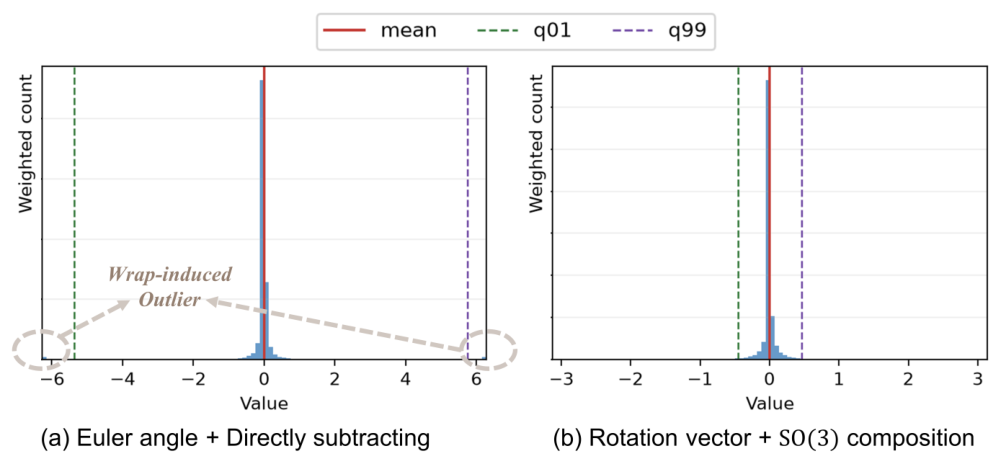
图 3:旋转动作分布的比较。(a) 用欧拉角表示并直接相减得到相对旋转目标。(b) 用旋转向量表示并通过 \mathrm{SO}(3) 复合计算相对旋转。在 (a) 中,角度回绕在 \pm2\pi 附近产生离群值,拉宽了第 1 与第 99 百分位数之间的区间。这会在归一化后严重压缩典型动作值的范围,妨碍训练。
原图注:Comparison of rotational action distributions. (a) Euler-angle representations with direct subtraction for relative-rotation targets. (b) Rotation-vector representations with relative rotations computed through \mathrm{SO}(3) composition. In (a), angular wrapping produces outliers near \pm2\pi, which widen the interval between the 1st and 99th percentiles. This severely compresses the range of typical action values after normalization, hindering training.
图 3 解读
两幅直方图都是持续预训练语料中某个旋转动作分量的加权计数分布,横轴是数值(弧度),纵轴是加权计数(未标刻度)。红色实线是均值,绿色虚线是第 1 百分位数 q01,紫色虚线是第 99 百分位数 q99。(a) 欧拉角直接相减:绝大部分值集中在 0 附近(\pm0.5 以内),但在 \pm6 附近(即 \pm2\pi)各有一小撮回绕导致的离群值(灰色虚线圈出),它们把 q01 和 q99 拉到了约 -5.4 和 +5.7。(b) 旋转向量 + \mathrm{SO}(3) 复合:离群值消失,q01、q99 约为 \pm0.45,横轴范围也只到 \pm\pi。为什么这会“妨碍训练”?\pi_{0.5}/openpi 常用分位数归一化:把 [q01,q99] 线性映射到 [-1,1]。在 (a) 中,这个区间宽约 11 弧度,而典型动作只有 \pm0.5 弧度,归一化后被压缩到约 \pm0.09 的窄带里,网络输出的微小误差就对应很大的实际转动误差;在 (b) 中区间宽约 0.9,典型动作能占满归一化后的大部分范围。这张图直观地解释了为什么动作表示的细节会显著影响训练效果。
原文
A rotation vector has a unified physical meaning through its direction and magnitude, making it natural to normalize its three channels using a shared scale. However, our controlled experiments show that channel-wise normalization yields substantially better performance, and we therefore adopt this approach in our experiments.
译文
旋转向量通过其方向和模长具有统一的物理含义,因此用一个共享尺度来归一化它的三个通道是很自然的。然而,我们的受控实验表明,逐通道归一化的性能要好得多,因此我们在实验中采用了逐通道归一化。
解释
旋转向量的三个分量合在一起才有几何意义(方向是转轴),所以从“保持几何”的角度看,三个通道应该用同一个缩放系数,否则归一化后的向量方向会被扭曲。但实验结果相反:逐通道(每个分量用各自的 q01/q99)更好。一个可能的解释是:机械臂实际运动中三个旋转分量的幅度差别很大(例如绕竖直轴的转动常比绕水平轴的大),共享尺度会让幅度小的分量被压到很窄的范围,与图 3 的道理相同。正文说“好得多”,但没有给出具体数字。
原文
Large numbers of similar trajectories can dominate a mixed training corpus without adding comparable behavioral diversity. This is particularly relevant to scripted simulation data, where repeated executions may follow highly regular motion patterns. We reduce such redundancy by subsampling complete episodes within tasks, preserving the original temporal sampling rate of every retained trajectory.
译文
大量相似的轨迹可能主导混合训练语料,却并不带来相应的行为多样性。这一点对脚本生成的仿真数据尤为明显,因为重复执行往往遵循高度规则的运动模式。我们通过在任务内部对完整回合进行子采样来减少这种冗余,并保留每条被保留轨迹原有的时间采样率。
解释
注意是“按回合”丢弃,而不是在轨迹内部隔帧抽取:隔帧抽取会改变控制频率,使动作块对应的物理时长变化,与其他数据集不一致;整条丢弃则不影响保留下来的轨迹。
原文
For example, for InternData-A1, we retain 3% of episodes for selected tasks with highly repetitive trajectories, and 10% for the other tasks. For the pre-training subsets of RoboCasa365, we retain 0.5% of the MimicGen episodes and 15% of the composite episodes. These source-dependent and task-dependent retention rates bring episode counts closer to a comparable order of magnitude, reducing the dominance of a small number of scenes or tasks.
译文
例如,对于 InternData-A1,我们对选定的轨迹高度重复的任务保留 3% 的回合,其他任务保留 10%。对于 RoboCasa365 的预训练子集,我们保留 0.5% 的 MimicGen 回合和 15% 的组合任务回合。这些依赖于数据源和任务的保留率,使各部分的回合数更接近同一数量级,减少了少数场景或任务的主导地位。
解释
粗略估算一下影响:InternData-A1 原有 630K 回合,保留 3%–10% 后只剩约 19K–63K;RoboCasa365 的 MimicGen 部分保留 0.5%,原子任务子集正文没说降采样(推测全保留)。这样一来,表 1 中占回合数 74% 的两个仿真数据集,处理后很可能降到与 AgiBot、RoboCOIN 同一量级甚至更少。这意味着表 1 的“170 万回合、14,330 小时”与实际训练语料的规模相差很大,读者引用这一数字时应注意。“选定的任务”具体是哪些,正文没有列出。
原文
We focus on manipulation with two-finger grippers and exclude dexterous-hand data and trajectories involving robot-base motion. We additionally use action statistics to identify and remove data with anomalous arm-motion speeds. Where existing annotations are available (Ye et al., 2026), we remove idle frames in which both the robot and the scene remain stationary. Together, these filters keep the corpus aligned with the intended control setting and reduce uninformative or inconsistent supervision.
译文
我们专注于二指夹爪的操作,排除灵巧手数据和涉及机器人底盘运动的轨迹。我们还利用动作统计量识别并去除机械臂运动速度异常的数据。在已有标注可用的情况下(Ye et al., 2026),我们去除机器人和场景都静止不动的空闲帧。这些过滤共同使语料与预期的控制设定保持一致,并减少无信息或不一致的监督。
解释
这三类过滤对应图 1 左下角“数据过滤”的四个小图标(灵巧手、异常、底盘运动、空闲)。去掉空闲帧对流匹配策略尤其重要:示范开头和结尾常有几秒钟机器人不动,若保留,模型会学到“在某些状态下输出零动作”,部署时容易出现停滞。去掉底盘运动是因为本文的动作空间只有机械臂末端和夹爪,基座运动会使“相对基座的末端位姿”与真实世界中的运动不一致。
4实验(Experiments)
4.1实验设置(Experimental Setup)
原文
We evaluate SLA through benchmark-specific post-training on three simulation benchmarks, one real-world benchmark, and plenty real-world deployments. These evaluations cover robustness to visual and language perturbations, manipulation under scene variation, and applicability across robot embodiments.
译文
我们在三个仿真基准、一个真实世界基准和大量真实世界部署中,通过针对各基准的后训练来评估 SLA。这些评估涵盖对视觉和语言扰动的鲁棒性、场景变化下的操作,以及在不同机器人本体上的适用性。
解释
所有评估都遵循“同一个持续预训练检查点 \to 针对每个基准单独后训练 \to 在该基准上评测”的流程。因此每个基准上的 SLA 是不同的模型,比较的是“基础模型 + 后训练配方”的整体效果。
原文
LIBERO-Plus (Fei et al., 2025) tests robustness along seven perturbation dimensions: camera, robot, language, lighting, background, observation noise, and object layout. We post-train on the standard LIBERO demonstrations and evaluate the perturbed environments without additional training on LIBERO-Plus. Evaluation comprises 10,030 rollouts; the overall SR weights each dimension by its number of evaluation episodes.
译文
LIBERO-Plus(Fei et al., 2025)沿七个扰动维度测试鲁棒性:相机、机器人、语言、光照、背景、观测噪声和物体布局。我们在标准 LIBERO 示范上后训练,然后在扰动环境中评估,不在 LIBERO-Plus 上做额外训练。评估共包含 10,030 次试验;总体成功率(SR)按每个维度的评估回合数加权。
解释
LIBERO-Plus 的训练数据就是原版 LIBERO 的四个套件,测试时对相机视角、机器人初始关节、指令措辞、光照、背景纹理、图像噪声、物体位置施加扰动,所以它测的是零样本鲁棒性。“按回合数加权”意味着某些维度(回合多的)对总分影响更大,总分不等于七列的简单平均;例如 SLA 七列的简单平均是 88.3,而加权总分是 87.4。
原文
RoboTwin 2.0 (Chen et al., 2025a) contains 50 bimanual manipulation tasks. We jointly post-train on 50 clean demonstrations per task and evaluate each task for 100 trials in both the Clean2Clean and Clean2Random settings. Clean2Random introduces domain randomization to test generalization beyond the clean training conditions. We report the task-averaged SR for each setting and their equal-weight average.
译文
RoboTwin 2.0(Chen et al., 2025a)包含 50 个双臂操作任务。我们在每个任务 50 条干净示范上联合后训练,并在 Clean2Clean 和 Clean2Random 两种设定下各对每个任务评估 100 次。Clean2Random 引入领域随机化,用来测试在干净训练条件之外的泛化。我们报告每种设定的任务平均 SR,以及二者的等权平均。
解释
“Clean”指桌面整洁、背景和光照固定;“Random”指加入杂乱物体、随机背景纹理、光照和桌面高度变化。50 个任务 \times 100 次 \times 2 种设定 =10{,}000 次试验,单个任务的 SR 粒度为 1%,任务平均后粒度为 0.02%。SR 在 70% 附近时,单任务 100 次试验的标准误约为 4.6 个百分点,50 个任务平均后的标准误约为 0.65 个百分点(若各任务独立)。
原文
RoboCasa-Panda (Nasiriany et al., 2024) contains 24-task kitchen manipulation benchmark covering pick-and-place, articulated-object interaction, and appliance operation with a Panda robot. Our post-training uses 50 demonstrations per task. Each task is evaluated for 50 trials under each of three evaluation seeds, yielding 3,600 trials in total. Results are averaged over seeds and tasks.
译文
RoboCasa-Panda(Nasiriany et al., 2024)是一个含 24 个任务的厨房操作基准,用 Panda 机器人完成抓放、铰接物体交互和电器操作。我们的后训练每个任务使用 50 条示范。每个任务在三个评估种子下各评估 50 次,共 3,600 次试验。结果对种子和任务取平均。
解释
24\times50\times3=3{,}600,与原文一致。“三个评估种子”指环境初始化(厨房布局、物体摆放)的随机种子,而不是训练种子;模型只训练了一次。RoboCasa 的示范来自人类遥操作,每任务 50 条是它官方提供的“人类示范”规模,其他方法常用 MimicGen 扩增到 300 或更多。
原文
RoboDojo-Real (Chen et al., 2026b) covers 18 tasks across ARX X5, Piper, and Piper X, with six tasks per embodiment. We jointly post-train a single model on demonstrations from all three embodiments. We report scores on a 0–100 scale to measure partial task progress and success rates to measure complete task success. Aggregation equally weights tasks within each embodiment and then the three embodiments.
译文
RoboDojo-Real(Chen et al., 2026b)涵盖 ARX X5、Piper 和 Piper X 三种本体上的 18 个任务,每种本体 6 个任务。我们在三种本体的全部示范上联合后训练一个模型。我们报告 0–100 分制的得分(Score)以衡量部分任务进度,并报告成功率以衡量完整的任务成功。汇总时先在每种本体内对任务等权平均,再对三种本体等权平均。
解释
RoboDojo 是一个公开的真机评测平台:参赛方提交模型,由平台方在其真机上统一评测,结果进入排行榜(表 5 中其他方法的数字即来自排行榜)。得分按任务阶段给部分分,比成功率更细。表 5 中每种本体的 SR 都是 1.7 的倍数(如 1.7、3.3、5.0、8.3),说明每种本体共 60 次试验,即每个任务 10 次;由此推算单任务 SR 的粒度为 10%,本体级 SR 在 30% 附近的标准误约为 6 个百分点。
原文
Apart from these benchmark evaluation, we additionally conduct real-world deployment experiments under eight private deployment conditions A–H on a bimanual Piper platform and a single-arm Franka robot. Piper platform uses one main camera and two wrist cameras while Franka uses one main camera and one wrist camera. The type of All cameras is Realsense D435. For each method, we post-train one policy on 100 demonstrations of A and reuse it for A–C evaluation. For D, we jointly post-train on the 100 Piper demonstrations of A and 10 additional Franka demonstrations. For task E–H, one policy is post-trained on 100 demonstrations collected in the E scene configuration and evaluated across E–H. We report object-level successs rates over 50 evaluated object instances per method and condition. For A, B, and D, these instances come from 10 rollouts with five objects per rollout, and each object is scored separately. C and E–H each comprise 50 single-object rollouts. Success requires complete manipulation sequence for the evaluated object.
译文
除这些基准评估外,我们还在一个双臂 Piper 平台和一台单臂 Franka 机器人上,于八种自建部署条件 A–H 下进行了真实世界部署实验。Piper 平台使用一个主相机和两个腕部相机,Franka 使用一个主相机和一个腕部相机。所有相机均为 RealSense D435。对每种方法,我们在条件 A 的 100 条示范上后训练一个策略,并复用它评估 A–C。对于 D,我们在 A 的 100 条 Piper 示范和另外 10 条 Franka 示范上联合后训练。对于任务 E–H,在 E 场景配置下采集的 100 条示范上后训练一个策略,并在 E–H 上评估。我们报告物体级成功率:每种方法、每种条件评估 50 个物体实例。对于 A、B 和 D,这些实例来自 10 次试验、每次 5 个物体,每个物体单独计分。C 和 E–H 各包含 50 次单物体试验。成功要求对被评估物体完成完整的操作序列。
解释
这一段把八个条件的训练—测试关系交代清楚了,可以整理成三组:A–C 共用一个双臂 Piper 策略(训练只见过 A);D 单独一个策略,训练用 100 条 Piper + 10 条 Franka,测试在 Franka 上;E–H 共用一个策略(训练只见过 E 场景)。因此 B、C、F、G、H 都是对未训练过的扰动的零样本测试。统计口径要注意:A、B、D 的“50 个实例”实际上是 10 次试验 \times 5 个物体,同一次试验内的 5 个物体结果高度相关(例如一开始抓偏,后面可能全失败),有效样本量更接近 10 而不是 50。即使按 50 个独立样本算,SR 在 80% 附近的标准误也约为 \sqrt{0.8\times0.2/50}\approx5.7 个百分点。所有真机实验均为单次评估,没有重复或置信区间。另外,所有相机都是能输出深度的 D435,但本文方法只用其 RGB。
4.2实现细节(Implementation Details)
原文
We initialize SLA from the pretrained \pi_{0.5} policy (Physical Intelligence, 2025) to conduct continual pre-training, followed by post-training for specific tasks.The continual pre-training runs for 36k optimizer steps with an effective global batch size of 4,608, obtained by accumulating gradients over two microsteps with a global batch size of 2,304 each. The learning rate warms up to 5\times10^{-5} over the first 1k steps, follows cosine decay to 1\times10^{-5} at step 30k, and remains constant thereafter. Continual pre-training takes approximately 110 hours on 48 NVIDIA H100 GPUs.
译文
我们用预训练好的 \pi_{0.5} 策略(Physical Intelligence, 2025)初始化 SLA,进行持续预训练,随后针对具体任务进行后训练。持续预训练共进行 36k 个优化步,有效全局批大小为 4,608,由两个微步的梯度累积得到,每个微步的全局批大小为 2,304。学习率在前 1k 步内预热到 5\times10^{-5},随后按余弦衰减,在第 30k 步降到 1\times10^{-5},此后保持不变。持续预训练在 48 块 NVIDIA H100 GPU 上耗时约 110 小时。
解释
算一下规模:2{,}304/48=48,即每块 GPU 每个微步 48 个样本;总样本数 36{,}000\times4{,}608\approx1.66\times10^8。计算量为 48\times110\approx5{,}280 GPU 小时。作为对照,若持续预训练语料按 30 Hz、14,330 小时计约有 1.5\times10^9 帧,训练只覆盖其约 11%;但正如第 3.3.2 节所说,实际用的是降采样后的子集,真实的“遍数”无法从正文推算。这一段也没有交代各数据集的混合采样比例。
原文
As for post-training, LIBERO-Plus takes 512 batch size and 30k steps, RoboTwin takes 256 batch size and 30k steps, RoboCasa-Panda takes 64 batch size and 60k steps, RoboDojo-Real takes 512 batch size and 40k steps, and all real-world deployment experiments take 64 batch size and 20k steps.
译文
后训练方面,LIBERO-Plus 使用 512 的批大小训练 30k 步,RoboTwin 使用 256 的批大小训练 30k 步,RoboCasa-Panda 使用 64 的批大小训练 60k 步,RoboDojo-Real 使用 512 的批大小训练 40k 步,所有真实世界部署实验都使用 64 的批大小训练 20k 步。
解释
真机部署实验每个策略只有 100 条(或 110 条)示范,却训练 64\times20{,}000=1.28\times10^6 个样本,按每条示范几百帧估算相当于数十遍数据,过拟合风险不小,这也许是状态丢弃在真机上有帮助的原因之一。正文没有说明基线(\pi_{0.5}、Spatial Forcing、OpenVLA-OFT、SpatialVLA)的后训练是否使用了相同的步数和批大小,也没有说明基线是否也用了状态丢弃。
4.3与最先进方法的比较(Comparisons with State-of-The-Art Methods)
原文
We compare against the methods listed in the benchmark tables. Spatial Forcing denotes our original method applied only during post-training from pretrained \pi_{0.5}, without our continual pre-training stage.
译文
我们与各基准表中列出的方法进行比较。Spatial Forcing 指我们的原始方法:只在从预训练 \pi_{0.5} 出发的后训练中使用,没有我们的持续预训练阶段。
解释
这一句给出了 Spatial Forcing 行的确切含义:\pi_{0.5} + 后训练对齐,没有持续预训练。它与 SLA 的差别因此是“持续预训练(含对齐)”加上配套部件(OmniVGGT 教师、门控多层、状态丢弃、统一动作表示)。表 2–4 和表 11 中 SF 行是作者自己跑的(灰底),其余基线大多来自原论文或排行榜。
4.3.1LIBERO-Plus
表 2:LIBERO-Plus 基准成功率(%,\uparrow)。模型在标准 LIBERO 训练集上微调,不使用 LIBERO-Plus 数据。平均值按评估回合数加权。粗体和下划线分别表示所列数值中的最佳和次佳。
| 方法 | 相机 | 机器人 | 语言 | 光照 | 背景 | 噪声 | 布局 | 平均 |
| \pi_0(Black et al., 2025) | 13.8 | 6.0 | 58.8 | 85.0 | 81.4 | 79.0 | 68.9 | 53.6 |
| \pi_{0.5}(Physical Intelligence, 2025) | 78.4 | 73.6 | 80.8 | 96.2 | 94.1 | 89.0 | 84.5 | 84.4 |
| StarVLA(Community, 2026) | 52.5 | 49.8 | 88.5 | 95.7 | 95.7 | 73.0 | 76.9 | 74.1 |
| 4D-WAM(Yang et al., 2026a) | 45.1 | 64.3 | 90.6 | 94.3 | 57.7 | 69.1 | 79.2 | 71.0 |
| Abot-M0(Yang et al., 2026c) | 60.4 | 67.9 | 86.4 | 96.2 | 91.6 | 86.4 | 82.6 | 80.5 |
| Cosmos Policy(Kim et al., 2026) | 75.8 | 63.3 | 81.7 | 96.5 | 88.9 | 92.7 | 82.2 | 82.2 |
| Being-H0.7(Luo et al., 2026) | 82.0 | 59.0 | 82.8 | 97.8 | 90.0 | 93.5 | 88.5 | 84.8 |
| Qwen-RobotManip(仅机器人数据)(Yuan et al., 2026b) | 72.8 | 78.2 | 88.7 | 97.5 | 97.6 | 95.4 | 85.4 | 87.1 |
| Spatial Forcing | 70.2 | 79.3 | 85.6 | 96.8 | 96.2 | 86.0 | 88.3 | 85.1 |
| SLA(本文) | 82.2 | 73.8 | 83.5 | 98.8 | 98.0 | 95.4 | 86.2 | 87.4 |
原表注:LIBERO-Plus benchmark success rates (%, \uparrow). Models are fine-tuned on the standard LIBERO training set without LIBERO-Plus set. Average is weighted by the number of evaluation episodes. Bold and underline denote the best and second-best displayed values, respectively.
表 2 解读
每行是一个方法,七列是七种扰动下的成功率,最后一列是按回合数加权的总分。灰底两行是作者团队的方法。SLA 的优势集中在视觉类扰动:相机(82.2,最高)、光照(98.8,最高)、背景(98.0,最高)、噪声(95.4,并列最高)。这与“空间对齐让视觉表征更关注几何结构、对外观变化更不敏感”的解释吻合。SLA 的弱项是机器人初始状态(73.8,比 SF 的 79.3 低 5.5)、语言(83.5,比 SF 低 2.1、比 4D-WAM 低 7.1)和布局(86.2,比 SF 低 2.1)。也就是说,加上持续预训练后,七个维度中有三个反而不如只做后训练对齐的 SF。机器人初始状态这一项尤其值得注意:持续预训练中使用了状态丢弃,理论上应减少对状态的依赖、提高对初始关节扰动的鲁棒性,但结果并非如此。总分 87.4 对第二名 Qwen-RobotManip 的 87.1 只领先 0.3 个百分点;在约 1 万次试验下,总分的标准误约为 \sqrt{0.87\times0.13/10030}\approx0.34 个百分点,这一差距在统计上不显著。
原文
Tab. 2 shows that SLA achieves a weighted SR of 87.4%, improving over \pi_{0.5} and Spatial Forcing by 3.0 and 2.3 percentage points, respectively. It exceeds the robot-only Qwen-RobotManip model (Yuan et al., 2026b) by 0.3 percentage points. Relative to the baseline \pi_{0.5}, improvements occur in all seven perturbation dimensions, including observation noise (89.0% to 95.4%) and background changes (94.1% to 98.0%). SLA also achieves the highest lighting-perturbation SR among the compared methods, at 98.8%. These results indicate that the benefits extend across a range of perturbations. These gains may stem in part from spatially informed visual representations that help the policy preserve task-relevant scene structure under challenging observation perturbations.
译文
表 2 显示,SLA 取得 87.4% 的加权 SR,比 \pi_{0.5} 和 Spatial Forcing 分别高 3.0 和 2.3 个百分点,比仅用机器人数据的 Qwen-RobotManip 模型(Yuan et al., 2026b)高 0.3 个百分点。相对于基线 \pi_{0.5},七个扰动维度全部有所提升,包括观测噪声(从 89.0% 到 95.4%)和背景变化(从 94.1% 到 98.0%)。SLA 在光照扰动下也取得了所比较方法中最高的 SR,为 98.8%。这些结果表明,收益覆盖了多种扰动。这些提升可能部分来自带有空间信息的视觉表征,它们帮助策略在具有挑战性的观测扰动下保留与任务相关的场景结构。
解释
文中数字都能在表中核对:87.4-84.4=3.0,87.4-85.1=2.3,87.4-87.1=0.3。“七个维度全部提升”相对 \pi_{0.5} 成立,但机器人维度只从 73.6 到 73.8(+0.2),相当于没有变化。文字只拿 \pi_{0.5} 作参照,回避了 SLA 在三个维度上不如 SF 的事实。最后一句用了“may stem in part from”,措辞是谨慎的:这是一种解释而非被验证的机制。
4.3.2RoboTwin
表 3:RoboTwin 2.0 基准成功率(%,\uparrow)。模型在 50 个标准任务上联合微调,每个任务使用 50 条 Clean 设定下的示范。逐任务结果见表 12。粗体和下划线表示所列数值中的最佳和次佳,并列者同等对待。
| 方法 | Clean2Clean | Clean2Random | 平均 |
| Discrete Forcing(Wang et al., 2026c) | 59.3 | 11.2 | 35.3 |
| X-WAM(Guo et al., 2026a) | 70.0 | 25.8 | 47.9 |
| \pi_{0.5}(Physical Intelligence, 2025) | 70.7 | 46.0 | 58.3 |
| 4D-WAM(Yang et al., 2026a) | 81.5 | 41.8 | 61.7 |
| WorldScape Policy 2.0(Su et al., 2026a) | 84.9 | 38.5 | 61.7 |
| GigaBrain-0.7(Team et al., 2026a) | 66.8 | 67.9 | 67.4 |
| UniWAM(Chen et al., 2026a) | 75.1 | 67.6 | 71.3 |
| ViGAR(Gong et al., 2026) | 82.0 | 67.0 | 74.5 |
| ME-Dex-1.0(Zhang et al., 2026) | 89.6 | 68.1 | 78.9 |
| Spatial Forcing | 74.7 | 62.6 | 68.7 |
| SLA(本文) | 86.0 | 72.3 | 79.2 |
原表注:RoboTwin 2.0 benchmark success rates (%, \uparrow). Models are fine-tuned jointly on the 50 standard tasks using 50 demonstrations from the Clean setting per task. Per-task results are shown in Tab. 12. Bold and underline denote the best and second-best displayed values, with ties treated equally.
表 3 解读
两列分别是在干净场景(与训练分布一致)和随机化场景(杂物、纹理、光照随机)中的平均成功率,第三列是二者的等权平均。方法大体按平均值从低到高排列。一个显著的现象是:多数方法从 Clean2Clean 到 Clean2Random 掉得很厉害(Discrete Forcing 从 59.3 掉到 11.2,WorldScape 从 84.9 掉到 38.5),说明它们对训练场景外观过拟合。少数方法(GigaBrain-0.7、UniWAM、ViGAR)在 Random 下仍有 67% 左右,掉幅较小。SLA 的 Clean2Random 是 72.3%,为表中最高,掉幅为 13.7 个百分点;SF 掉 12.1,\pi_{0.5} 掉 24.7。对齐(无论是否有持续预训练)明显减小了这一掉幅。在 Clean2Clean 上 SLA(86.0)不如 ME-Dex-1.0(89.6),平均值也只领先 0.3(79.2 对 78.9)。SLA 相对 SF 的提升(平均 +10.5)比相对最强外部基线的提升大得多,这一对比才是本表对本文主张最有力的支持。\pi_{0.5} 的 Clean2Random 为 46.0%,就是图 4 中的虚线基准。
原文
Tab. 3 shows that SLA achieves 86.0% Clean2Clean SR, 72.3% Clean2Random SR, and a 79.2% average on RoboTwin 2.0. The Clean2Random and average results exceed \pi_{0.5} by 26.3 and 20.9 percentage points, respectively. Clean2Clean primarily assesses performance under conditions similar to the training demonstrations, whereas Clean2Random tests generalization under domain randomization and thus provides a more demanding measure of robustness to scene variation. Compared with ME-Dex-1.0 (Zhang et al., 2026), the strongest competing method by average SR in the table, SLA improves Clean2Random SR by 4.2 points while trailing its Clean2Clean SR. The average also exceeds the original Spatial Forcing method by 10.5 points, supporting the effectiveness of the complete training approach beyond post-training-only spatial alignment. The substantial gain in the Clean2Random setting suggests that SLA helps the policy generalize beyond the clean training conditions to more varied manipulation scenes.
译文
表 3 显示,SLA 在 RoboTwin 2.0 上取得 86.0% 的 Clean2Clean SR、72.3% 的 Clean2Random SR 和 79.2% 的平均值。其 Clean2Random 和平均结果分别比 \pi_{0.5} 高 26.3 和 20.9 个百分点。Clean2Clean 主要评估与训练示范相似条件下的性能,而 Clean2Random 测试领域随机化下的泛化,因而是对场景变化鲁棒性更严格的衡量。与表中按平均 SR 最强的对比方法 ME-Dex-1.0(Zhang et al., 2026)相比,SLA 的 Clean2Random SR 高 4.2 个百分点,但 Clean2Clean SR 落后。其平均值还比原始的 Spatial Forcing 方法高 10.5 个百分点,支持了完整训练方法相对于仅在后训练中做空间对齐的有效性。Clean2Random 设定下的大幅提升表明,SLA 帮助策略泛化到干净训练条件之外更多样的操作场景。
解释
数字核对:72.3-46.0=26.3;79.2-58.3=20.9;72.3-68.1=4.2;79.2-68.7=10.5,均与表一致。文字坦承了 Clean2Clean 落后于 ME-Dex-1.0(落后 3.6)。需要指出的是,表 8 显示同一个持续预训练检查点在后训练时若不用状态丢弃,平均 SR 只有 38.1%,远低于 SF 的 68.7%;正文没有说明 SF 是否使用了状态丢弃。如果没有,那么“比 SF 高 10.5”中有一部分可能来自状态丢弃这一与持续预训练无关的训练技巧。
4.3.3RoboCasa-Panda
表 4:RoboCasa-Panda 基准成功率(%,\uparrow)。逐任务结果见表 13。粗体和下划线表示所列数值中的最佳和次佳。
| 方法 | 每任务训练示范数 | 平均 |
| GR00T-N1(Bjorck et al., 2025) | 300 | 49.6 |
| UVA(Li et al., 2025b) | 50 | 50.0 |
| DP-VLA(Han et al., 2024) | 3000 | 57.3 |
| DreamGen(Jang et al., 2025) | 300 | 57.6 |
| DUST(Won et al., 2025) | 300 | 58.5 |
| UWM(Zhu et al., 2025) | 1000 | 60.8 |
| \pi_0(Black et al., 2025) | 300 | 62.5 |
| GR00T-N1.5(NVIDIA, 2025) | 300 | 64.1 |
| Video Policy(Liang et al., 2025) | 300 | 66.0 |
| FLARE(Zheng et al., 2025b) | 300 | 66.4 |
| HAMLET(Koo et al., 2026) | 300 | 66.4 |
| Cosmos Policy(Kim et al., 2026) | 50 | 67.1 |
| Spatial Forcing | 50 | 67.6 |
| SLA(本文) | 50 | 68.4 |
原表注:RoboCasa-Panda benchmark success rates (%, \uparrow). Per-task results are shown in Tab. 13. Bold and underline denote the best and second-best displayed values.
表 4 解读
第二列是各方法下游训练时每个任务用的示范数,第三列是 24 个任务的平均成功率。从 49.6 到 68.4,大多数方法挤在 57–67 之间。同样只用 50 条示范的方法有三个外部对照:UVA(50.0)、Cosmos Policy(67.1),以及作者的 SF(67.6)。SLA 比 SF 高 0.8、比 Cosmos Policy 高 1.3 个百分点。按 3,600 次试验计,总平均的标准误约 \sqrt{0.684\times0.316/3600}\approx0.77 个百分点,因此 SLA 与 SF、Cosmos Policy 之间的差距都在一到两个标准误之内,算不上可靠的领先。用 300–3,000 条示范的方法普遍更低,主要说明它们的基础模型或架构与 \pi_{0.5} 系列有差距,或这些方法在更早的时间点发表,不宜直接解读为“SLA 的数据效率是它们的 6–60 倍”。另外,如第 3.3.1 节所述,SLA 的持续预训练语料包含 RoboCasa365 预训练子集,与本基准同平台。
原文
Tab. 4 shows that SLA reaches a mean success rate of 68.4% on RoboCasa-Panda, the highest result among the compared methods. It exceeds Cosmos Policy (Kim et al., 2026) by 1.3 percentage points and Spatial Forcing by 0.8 points, with all three using 50 post-training demonstrations per task. Other models use different demonstration budgets, as explicitly reported in the table. This comparison shows that our proposed approach remains competitive when adaptation data are limited. The task-specific breakdown in Tab. 13 shows that SLA achieves success rates above 80% on 10 of the 24 tasks, including 100.0% on TurnOffMicrowave.
译文
表 4 显示,SLA 在 RoboCasa-Panda 上的平均成功率达到 68.4%,是所比较方法中的最高结果。它比 Cosmos Policy(Kim et al., 2026)高 1.3 个百分点,比 Spatial Forcing 高 0.8 个百分点,三者每个任务都使用 50 条后训练示范。其他模型使用不同的示范数量,表中已明确列出。这一比较表明,在适配数据有限时,我们提出的方法仍具竞争力。表 13 的逐任务结果显示,SLA 在 24 个任务中的 10 个上成功率超过 80%,其中 TurnOffMicrowave(关微波炉)达到 100.0%。
解释
这一段的措辞(“remains competitive”)比摘要中的“state-of-the-art”和引言中的“exceeding compared policies trained with 300–3,000 demonstrations”更克制,也更符合 0.8 个百分点的实际差距。“10 个任务超过 80%”可以在附录表 13 中核对(见本译稿“附录概览”)。
4.3.4RoboDojo-Real
表 5:三种本体上的 RoboDojo 真实世界基准结果。得分(\uparrow)反映部分任务进度,SR(%,\uparrow)衡量二元的任务完成。逐任务结果见表 14。粗体和下划线表示所列数值中的最佳和次佳。
| 方法 | ARX X5 | Piper | Piper X | 平均 | ||||
| 得分 | SR | 得分 | SR | 得分 | SR | 得分 | SR | |
| Spirit v1.5(Team, 2026) | 0.0 | 0.0 | 4.0 | 1.7 | 0.7 | 0.0 | 1.6 | 0.6 |
| StarVLA(Community, 2026) | 0.0 | 0.0 | 12.0 | 5.0 | 0.5 | 0.0 | 4.1 | 1.7 |
| \pi_0(Black et al., 2025) | 8.1 | 0.0 | 9.0 | 5.0 | 0.3 | 0.0 | 5.8 | 1.7 |
| GR00T-N1.7(Bjorck et al., 2025) | 9.3 | 1.7 | 6.8 | 3.3 | 1.4 | 0.0 | 5.9 | 1.7 |
| X-VLA(Zheng et al., 2025a) | 6.8 | 1.7 | 15.9 | 8.3 | 0.1 | 0.0 | 7.6 | 3.3 |
| Xiaomi-Robotics-0(Cai et al., 2026b) | 15.0 | 8.3 | 7.6 | 3.3 | 1.2 | 0.0 | 7.9 | 3.9 |
| GalaxeaVLA(Jiang et al., 2026) | 3.4 | 0.0 | 22.0 | 13.3 | 1.7 | 0.0 | 9.0 | 4.4 |
| InternVLA-A1(Cai et al., 2026a) | 10.0 | 3.3 | 23.2 | 18.3 | 2.7 | 0.0 | 12.0 | 7.2 |
| \pi_{0.5}(Physical Intelligence, 2025) | 27.7 | 13.3 | 32.0 | 21.7 | 9.1 | 3.3 | 22.9 | 12.8 |
| OpenWAM-\alpha(Wang et al., 2026e) | 39.0 | 23.3 | 46.7 | 36.7 | 27.2 | 13.3 | 37.6 | 24.4 |
| InternW0-\Delta(Miao et al., 2026) | 59.7 | 50.0 | 39.3 | 31.7 | 17.8 | 13.3 | 38.9 | 31.7 |
| SLA(本文) | 50.3 | 36.7 | 60.3 | 55.0 | 16.3 | 10.0 | 42.3 | 33.9 |
原表注:RoboDojo real-world benchmark results across three embodiments. Score (\uparrow) captures partial task progress, and SR (%, \uparrow) measures binary task completion. Per-task results are shown in Tab. 14. Bold and underline denote the best and second-best displayed values.
表 5 解读
三组列对应三种机械臂平台,每组有得分和成功率两列,最后一组是三种本体的等权平均。表的上半部分(\pi_{0.5} 以上)大多是通用 VLA,成功率基本在 0–8% 之间,说明 RoboDojo-Real 的任务很难;下面两个强基线 OpenWAM-\alpha 和 InternW0-\Delta 都是世界动作模型(WAM),本工作区有它们的译稿。平均值可以核对:SLA 得分 (50.3+60.3+16.3)/3=42.3,SR (36.7+55.0+10.0)/3=33.9;\pi_{0.5} SR (13.3+21.7+3.3)/3=12.8。SLA 的总分领先主要来自 Piper(SR 55.0,比次佳的 36.7 高 18.3);在 ARX X5 上它落后 InternW0-\Delta 13.3 个百分点;在 Piper X 上它的得分(16.3)只排第三,成功率(10.0)低于两个 WAM 的 13.3。所以“总体最强”是由一种本体上的大优势带来的,三种本体并非一致领先。还要注意本表的比较口径:其他方法的结果来自 RoboDojo 排行榜,而 SLA 在这一基准的后训练中额外加入了记忆机制(多帧历史图像输入,见附录 B),\pi_{0.5} 基线是否有同样的记忆输入并未说明,表中也没有 Spatial Forcing 这一行。因此本表无法区分提升来自空间对齐、持续预训练还是记忆机制。
原文
Tab. 5 evaluates whether our approach remains useful for real-world benchmarks, especially when a single policy is adapted jointly to several physical embodiments. To address long-horizon tasks and long-term memory requirements in RoboDojo-Real benchmark, we incorporate a memory mechanism into the policy during post-training, as detailed in Sec. B. SLA achieves the highest overall score and success rate among the compared methods at 42.3 and 33.9%, exceeding \pi_{0.5} by 19.4 score points and 21.1 percentage points, respectively. It also surpasses InternW0-\Delta (Miao et al., 2026), the strongest competing method overall, by 3.4 score points and 2.2 percentage points. On Piper, SLA leads in both metrics, with a Score of 60.3 and SR of 55.0%. On ARX X5, it ranks second in both metrics behind InternW0-\Delta. These results support the effectiveness of our training approach to joint multi-embodiment adaptation, highlighting its potential for real-world manipulation. The spatial alignment branch is used only during training, while the historical image inputs of the memory mechanism are retained at inference.
译文
表 5 评估我们的方法在真实世界基准上是否仍然有效,尤其是当一个策略被联合适配到多种实体本体时。为应对 RoboDojo-Real 基准中的长时程任务和长期记忆需求,我们在后训练中为策略加入了记忆机制,详见附录 B。SLA 取得了所比较方法中最高的总体得分和成功率,分别为 42.3 和 33.9%,比 \pi_{0.5} 分别高 19.4 分和 21.1 个百分点。它还以 3.4 分和 2.2 个百分点超过了总体最强的对比方法 InternW0-\Delta(Miao et al., 2026)。在 Piper 上,SLA 两项指标都领先,得分 60.3、SR 55.0%。在 ARX X5 上,它两项指标都排第二,仅次于 InternW0-\Delta。这些结果支持了我们的训练方法在多本体联合适配中的有效性,显示了其在真实世界操作中的潜力。空间对齐分支只在训练中使用,而记忆机制的历史图像输入在推理时保留。
解释
数字核对:42.3-22.9=19.4,33.9-12.8=21.1,42.3-38.9=3.4,33.9-31.7=2.2,均一致。文字只提了 Piper 和 ARX X5,没有提 SLA 表现最弱的 Piper X。最后一句是重要的限定:前文反复强调“推理架构与 \pi_{0.5} 完全相同”,但在 RoboDojo-Real 上并非如此,部署的模型多了历史图像输入,推理时的 token 数和计算量都会增加。这一点在摘要和引言中都没有提及。记忆机制的具体做法只在附录 B 中给出(本译稿的“附录概览”有简述)。
4.4性能分析(Performance Analysis)
4.4.1数据扩展趋势(Data Scaling Trend)
表 6:持续预训练数据扩展消融。SLA 对齐在持续预训练和后训练中分别独立开启或关闭。对应的折线图见图 4。实验在 RoboTwin Clean2Random 设定下进行,评估成功率(%,\uparrow)。
| SLA 对齐 | 持续预训练数据(%) | ||||
| 预训练 | 后训练 | 5 | 25 | 50 | 100 |
| ✗ | ✗ | 43.8 | 46.5 | 46.1 | 48.2 |
| ✗ | ✓ | 45.6 | 53.4 | 55.3 | 57.1 |
| ✓ | ✗ | 46.6 | 52.0 | 58.4 | 63.2 |
| ✓ | ✓ | 49.2 | 60.5 | 67.4 | 72.3 |
原表注:Continual pre-training data scaling ablation. SLA alignment is independently enabled or disabled during continual pre-training and post-training. The corresponding line chart is plotted in Fig. 4. Experiments are conducted under the RoboTwin Clean2Random settings to evaluate success rates (%, \uparrow).
表 6 解读
这是本文最核心的对照实验,设计为 2\times2\times4:持续预训练时是否对齐、后训练时是否对齐、持续预训练用多少比例的数据。四行对应四种对齐组合,四列是数据比例;所有数字都是 RoboTwin Clean2Random 50 个任务的平均 SR。行间比较(看对齐的作用):在 100% 数据下,四种组合依次是 48.2、57.1、63.2、72.3。只在预训练对齐(63.2)比只在后训练对齐(57.1)高 6.1,说明把对齐放进预训练更有价值;两阶段都对齐又比只在预训练对齐高 9.1,说明后训练继续对齐仍有增益。两者的增益大致可以叠加:48.2+(57.1-48.2)+(63.2-48.2)=72.1,与实测 72.3 几乎相同,说明两阶段对齐的作用近似独立、可加。列间比较(看数据量的作用):不对齐时从 5% 到 100% 只涨 4.4(43.8 \to 48.2),中间还有回落;两阶段都对齐时涨 23.1(49.2 \to 72.3)。也就是说,在没有对齐损失时,单纯在这批数据上做持续预训练几乎没有用,对齐损失才让数据量的增加转化成下游收益。这是本文“扩展空间对齐”这一主张最直接的证据。但这张表也有令人困惑的地方,见图 4 的解读。
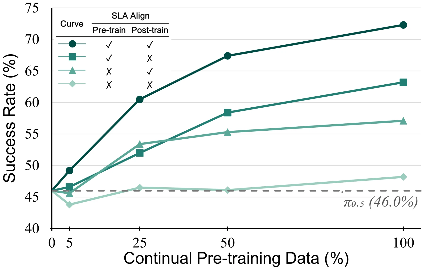
图 4:持续预训练数据扩展消融。SLA 对齐在持续预训练和后训练中分别独立开启或关闭。所有曲线都从共同的 \pi_{0.5} 基线出发。实验在 RoboTwin Clean2Random 设定下进行,评估成功率(%,\uparrow)。
原图注:Continual pre-training data scaling ablation. SLA alignment is independently enabled or disabled during continual pre-training and post-training. All curves start at the shared \pi_{0.5} baseline. Experiments are conducted under RoboTwin Clean2Random settings to evaluate success rates (%, \uparrow).
图 4 解读
这是表 6 的折线图。横轴是持续预训练数据比例(0、5、25、50、100%,注意横轴是线性刻度,所以 0 和 5 挤在一起),纵轴是 Clean2Random 成功率。图例中圆点、方块、三角、菱形分别对应“两阶段都对齐”“只预训练对齐”“只后训练对齐”“都不对齐”,颜色由深到浅。灰色虚线是 \pi_{0.5} 的 46.0%。四条曲线在 0% 处都画在 46.0%,即“不做持续预训练”的起点被设为 \pi_{0.5}。这对“预训练对齐”的两条曲线没有问题(0% 数据时预训练对齐没有意义)。但对“只后训练对齐”(三角)这条曲线,0% 数据时的配置就是“\pi_{0.5} + 后训练对齐”,也就是 Spatial Forcing,而表 3 中 SF 的 Clean2Random 是 62.6%,不是 46.0%。按表 3 的数字,三角曲线应从 62.6 出发,经过 5% 时的 45.6 和 100% 时的 57.1,即持续预训练(不对齐)后再做后训练对齐,在所有数据比例下都不如完全不做持续预训练的 SF。原文没有解释这一矛盾。可能的原因包括:本消融的后训练设置(步数、状态丢弃、动作表示)与表 3 中 SF 的设置不同;或持续预训练改变了动作空间约定(统一的 EEF 增量表示),使后续在 RoboTwin 上的适配需要更多步数。无论哪种,图中“所有曲线从共同的 \pi_{0.5} 出发”的画法都掩盖了这一点。类似地,“都不对齐”的菱形曲线在 5% 数据时(43.8)低于起点 46.0,说明少量持续预训练反而有害,这与上面的现象一致:持续预训练本身在不加对齐时价值有限甚至为负。
原文
A key question for continual pre-training is whether additional training data translate into better downstream performance. To examine this relationship, we sample demonstrations within each task of the full pre-training mixture to construct subsets containing 5%, 25%, 50%, and 100% of the original data. For each subset, we perform continual pre-training with and without SLA alignment to obtain separate checkpoints. We then independently enable or disable alignment during post-training to examine how spatial supervision in the two stages interacts, yielding the four configurations shown in Tab. 6 and Fig. 4.
译文
持续预训练的一个关键问题是:更多的训练数据能否转化为更好的下游性能。为考察这一关系,我们在完整预训练混合数据的每个任务内对示范进行采样,构造包含原始数据 5%、25%、50% 和 100% 的子集。对每个子集,我们分别在有和没有 SLA 对齐的情况下进行持续预训练,得到不同的检查点。随后我们在后训练中独立地开启或关闭对齐,以考察两个阶段的空间监督如何相互作用,得到表 6 和图 4 所示的四种配置。
解释
实验设计共需 4\times2=8 次持续预训练(每次 36k 步、约 110 小时、48 块 H100 的话共约 4 万 GPU 小时)和 16 次后训练。正文没有说明不同数据比例下持续预训练的步数是否相同。如果步数相同(都是 36k),那么 5% 子集会被重复很多遍、100% 子集只过一遍左右,“数据量”与“重复次数”是混在一起变化的;如果步数按比例缩减,则“数据量”与“训练计算量”混在一起。两种情况下曲线的解读不同,原文未交代。“在每个任务内采样”保证了各子集的任务覆盖相同,只是每任务的示范数不同。
原文
We report RoboTwin 2.0 Clean2Random SR averaged over all 50 tasks. With SLA alignment in both stages, SR increases from 49.2% at 5% data to 72.3% at full data, a gain of 23.1 percentage points. This configuration performs best at every tested proportion. Without alignment in either stage, SR changes from 43.8% to 48.2%, with a small decline between 25% and 50% data. Increasing data alone therefore provides a much smaller benefit in this comparison.
译文
我们报告 RoboTwin 2.0 Clean2Random 下 50 个任务的平均 SR。两阶段都使用 SLA 对齐时,SR 从 5% 数据时的 49.2% 提高到全量数据时的 72.3%,提升 23.1 个百分点;这一配置在每个测试比例下都表现最好。两阶段都不对齐时,SR 从 43.8% 变为 48.2%,且在 25% 到 50% 数据之间略有下降。因此在这一比较中,仅增加数据带来的收益要小得多。
解释
数字核对:72.3-49.2=23.1;不对齐时 25% 为 46.5、50% 为 46.1,确有 0.4 的回落(在约 0.7 个百分点的标准误之内,可视为持平)。“Increasing data alone provides a much smaller benefit”是对“都不对齐”这一行的准确概括。曲线在 50% 到 100% 之间仍在上升(67.4 \to 72.3),尚未饱和,暗示继续扩数据可能还有收益,但只有四个数据点,不足以拟合扩展律。
原文
The two single-stage variants further clarify the role of spatial supervision. At full data, SLA alignment only during continual pre-training reaches 63.2%, compared with 57.1% when applied only during post-training. Applying alignment in both stages improves on these variants by 9.1 and 15.2 percentage points, respectively. Overall, the consistently stronger joint configuration supports using spatial supervision both to shape the pretrained representation and to guide its downstream adaptation.
译文
两种单阶段变体进一步阐明了空间监督的作用。在全量数据下,只在持续预训练中使用 SLA 对齐达到 63.2%,而只在后训练中使用时为 57.1%。两阶段都使用对齐比这两种变体分别高 9.1 和 15.2 个百分点。总的来说,联合配置始终更强,支持了既用空间监督塑造预训练表征、又用它引导下游适配的做法。
解释
72.3-63.2=9.1,72.3-57.1=15.2,与表一致。在 25% 数据处两种单阶段变体的排序与其他比例相反(只后训练对齐 53.4 > 只预训练对齐 52.0),差距只有 1.4,属于噪声范围。正如图 4 解读中指出的,“只后训练对齐”这一行在各个数据比例下都低于表 3 中不做持续预训练的 SF(62.6),这意味着就后训练对齐而言,先在这批数据上不对齐地持续预训练是有害的;这一点在正文中没有讨论。
4.4.2自适应层选择(Adaptive Layer Selection)
表 7:自适应层选择消融。固定层变体只用 VLA 某一个 Transformer 层的视觉 token 做对齐;自适应变体使用学到的融合机制。实验在 RoboTwin 上进行,评估成功率(%,\uparrow)。
| 对齐层 | Clean2Clean | Clean2Random | 平均 |
| 1 | 60.0 | 43.4 | 51.7 |
| 6 | 63.0 | 45.0 | 54.0 |
| 12 | 84.0 | 67.3 | 75.7 |
| 18 | 78.0 | 64.6 | 71.3 |
| 自适应 | 86.0 | 72.3 | 79.2 |
原表注:Adaptive layer selection ablation. Fixed variants use visual tokens from a single VLA transformer layer for alignment; Adaptive variants use the learned fusion mechanism. Experiments are conducted on RoboTwin to evaluate success rates (%, \uparrow).
表 7 解读
行是对齐所用的层:Gemma 主干 18 层中的第 1、6、12、18 层,以及在全部 18 层上自适应融合。列与表 3 相同。规律很清楚:对齐太浅(第 1、6 层)效果很差,平均只有 51.7、54.0,甚至低于不做任何对齐的 \pi_{0.5}(58.3);中间偏深的第 12 层最好(75.7);最深的第 18 层又略降(71.3)。自适应融合比最好的单层再高 3.5(平均)和 5.0(Clean2Random)。需要弄清的是这张表的实验协议:自适应一行的数字与主结果(表 3)完全相同,说明它就是完整的 SLA。那么固定层的变体是在持续预训练和后训练中都改用固定层,还是只在后训练中改?如果持续预训练也要重做,每一行就是一次 5,000 GPU 小时级的训练;正文没有说明。若只在后训练中改层,而持续预训练用的是自适应融合,那么固定层变体在后训练时对齐的层与预训练时形成的表征并不匹配,这对固定层变体不利。另外,第 1、6 层的结果低于 \pi_{0.5},说明对齐错误的层会损害性能,选层不是无关紧要的超参数。
原文
A fixed alignment layer requires manual selection and may not suit different data domains. We therefore introduce the adaptive layer selection mechanism to learn each layer's contribution to spatial supervision, as explained in Sec. 3.2.3. Specifically, our PaliGemma VLM (Beyer et al., 2024) has 18 transformer layers in its language backbone. We compare single-layer alignment at layers 1, 6, 12, and 18 with adaptive fusion across all 18 layers. In Tab. 7, fixed-layer Clean2Random success rates range from 43.4% to 67.3%. Layer 12 performs best, while layer 18 drops to 64.6%, showing that deeper alignment is not necessarily better. Adaptive fusion achieves 72.3% Clean2Random success rates and 79.2% average success rates, exceeding layer 12 by 5.0 and 3.5 percentage points, respectively. This result supports learning the contributions of multiple layers instead of committing to a single layer depth. The improvement is consistent with the motivation for token- and channel-wise gating: allowing the spatial alignment signal to draw on features from different representation depths.
译文
固定的对齐层需要手动选择,而且可能不适合不同的数据域。因此,如第 3.2.3 节所述,我们引入自适应层选择机制来学习每一层对空间监督的贡献。具体而言,我们的 PaliGemma VLM(Beyer et al., 2024)的语言主干有 18 个 Transformer 层。我们把在第 1、6、12、18 层上的单层对齐与在全部 18 层上的自适应融合进行比较。在表 7 中,固定层的 Clean2Random 成功率在 43.4% 到 67.3% 之间。第 12 层表现最好,而第 18 层降到 64.6%,说明对齐越深不一定越好。自适应融合取得 72.3% 的 Clean2Random 成功率和 79.2% 的平均成功率,分别比第 12 层高 5.0 和 3.5 个百分点。这一结果支持学习多个层的贡献,而不是固定于单一层深度。这一提升与采用逐 token、逐通道门控的动机一致:让空间对齐信号能够利用来自不同表征深度的特征。
解释
数字核对:72.3-67.3=5.0,79.2-75.7=3.5。最后一句是“与动机一致”,而不是“证明了门控在按数据域选择不同的层”:要支持后者,需要展示不同数据域上门控权重确实不同,本文没有给出这种分析。还有一个更简单的对照没有做:对所有层等权平均(不用门控)。没有这个对照,就无法区分收益来自“多层一起对齐”还是来自“依赖于特征的门控”。
4.4.3状态丢弃(State Dropout)
表 8:状态丢弃消融。实验在 RoboTwin 上进行,评估成功率(%,\uparrow)。
| 状态丢弃概率 | Clean2Clean | Clean2Random | 平均 |
| 0% | 55.5 | 20.7 | 38.1 |
| 25% | 86.0 | 72.3 | 79.2 |
| 50% | 66.5 | 41.3 | 53.9 |
| 75% | 72.1 | 51.6 | 61.9 |
| 100% | 62.4 | 50.9 | 56.7 |
原表注:State dropout ablation. Experiments are conducted on RoboTwin to evaluate success rates (%, \uparrow).
表 8 解读
行是后训练时状态被整段丢弃的概率,0% 表示总是给状态,100% 表示从不给状态。所有行都从同一个持续预训练检查点出发。这张表的数字波动之大值得警惕。第一,不丢弃状态(0%)时平均只有 38.1%、Clean2Random 只有 20.7%,远低于 \pi_{0.5} 的 58.3/46.0 和 SF 的 68.7/62.6。也就是说,经过 SLA 持续预训练的检查点,如果后训练不用状态丢弃,会比原版 \pi_{0.5} 差很多。第二,概率与性能的关系极不平滑:25% 时 79.2,50% 时骤降到 53.9,75% 时又回升到 61.9,100% 时 56.7。一个正则化超参数在 25%、50%、75% 之间造成 25 个百分点的来回波动,很难用“视觉依赖与本体信息之间的平衡”解释,更像是训练不稳定或单次运行的方差很大。这对理解全文结论有直接影响:主表中 SLA 的 79.2 恰好是这条非单调曲线上的最高点;如果状态丢弃对结果的影响这么大,那么 SF 和 \pi_{0.5} 基线是否使用了状态丢弃、是否也做了类似的调参,就成为公平比较的关键,而正文没有说明。另外,正文说状态丢弃在“两个训练阶段”都使用,但这里只扫了后训练阶段的概率,持续预训练阶段的概率未给出。
原文
State dropout is intended to discourage shortcuts based on associations between robot states and demonstrated trajectories, encouraging the policy to encode scene geometry and use visual observations for action generation. To assess its effect on manipulation performance, we vary the state dropout probability during post-training, starting from the same continually pretrained checkpoint and evaluating all 50 RoboTwin tasks. As shown in Tab. 8, 25% dropout achieves the best average SR of 79.2%, compared with 38.1% without dropout. It also yields the highest Clean2Clean and Clean2Random results. Larger dropout probabilities perform less well: even 75%, the next-best setting, reaches only 61.9% on average. The response is not monotonic, and removing state inputs from every training sample is also suboptimal. These observations favor partial state dropout, consistent with a balance between encouraging reliance on visual evidence and preserving access to proprioceptive information during training.
译文
状态丢弃旨在抑制基于“机器人状态—示范轨迹”关联的捷径,促使策略编码场景几何并利用视觉观测生成动作。为评估它对操作性能的影响,我们从同一个持续预训练检查点出发,在后训练中改变状态丢弃概率,并在全部 50 个 RoboTwin 任务上评估。如表 8 所示,25% 的丢弃率取得最佳平均 SR 79.2%,而不丢弃时为 38.1%。它在 Clean2Clean 和 Clean2Random 上也都取得最高结果。更大的丢弃概率表现较差:即使是次佳的 75%,平均也只有 61.9%。这种响应不是单调的,而且在每个训练样本中都去掉状态输入同样不是最优。这些观察支持部分状态丢弃,与“既鼓励依赖视觉证据、又在训练中保留本体感知信息”之间的平衡相一致。
解释
文字承认了响应“不单调”,但没有讨论 50% 处的骤降。值得思考的是 0% 时的崩溃:同样的 RoboTwin 数据、同样不丢状态,\pi_{0.5} 能达到 58.3,经过持续预训练后的检查点只有 38.1。一种可能是持续预训练中一直使用状态丢弃,模型已习惯“有时没有状态”,后训练突然 100% 给状态反而形成新的捷径;另一种可能是持续预训练统一后的状态表示(EEF 绝对位姿)与 RoboTwin 的状态分布差别大,使状态输入更容易被过拟合。作者没有给出分析。
4.4.4旋转表示(Rotation Representation)
表 9:旋转表示消融。所有变体都通过 \mathrm{SO}(3) 复合而非直接相减来计算相对旋转,以避免回绕导致的离群值,详见式 (10)。实验在 RoboTwin 上进行,评估成功率(%,\uparrow)。
| 旋转表示 | Clean2Clean | Clean2Random | 平均 |
| 欧拉角 | 71.6 | 59.3 | 65.5 |
| Rot6D | 66.9 | 58.8 | 62.9 |
| 四元数 | 81.1 | 67.5 | 74.3 |
| 旋转向量 | 86.0 | 72.3 | 79.2 |
原表注:Rotation representation ablation. All variants compute relative rotations through \mathrm{SO}(3) composition rather than direct subtraction to avoid wrap-induced outliers, as detailed in Eq. (10). Experiments are conducted on RoboTwin to evaluate success rates (%, \uparrow).
表 9 解读
四行是四种表示 \Delta R_t 的方式,相对旋转都已经用 \mathrm{SO}(3) 复合算好,区别只在于把这个相对旋转写成哪几个数让网络去预测。旋转向量(3 维)最好,四元数(4 维)次之,欧拉角(3 维)和 Rot6D(6 维)明显较差,最好与最差相差 16.3 个百分点(平均)。Rot6D 在学术界常被推荐为“连续、适合神经网络回归”的表示(Zhou et al., CVPR 2019),这里却最差,这是一个有些反直觉的结果。一个可能的解释是:动作块里的相对旋转通常很小,在小角度下旋转向量近似线性、各分量相互独立,非常适合回归;而 Rot6D 在零旋转附近的 6 个分量中有 2 个接近 1、其余接近 0,归一化后有效信息被压缩。需要注意,这里的“欧拉角”已经不是图 3 中直接相减的那种,因此它与旋转向量的差距(13.7)不能归因于回绕离群值。与表 7、表 8 一样,正文没说明这些变体是否也重做了持续预训练;如果只改后训练的旋转表示,那么非旋转向量的变体就在用一种与预训练时不同的动作空间做微调,对它们不利。
原文
Because our action space is defined in terms of end-effector poses, the rotation representation determines how orientation changes are encoded as action targets. We compare four rotation representations during post-training from the same continually pretrained checkpoint on all 50 RoboTwin tasks. Tab. 9 shows that rotation vectors achieve the highest average SR of 79.2%, followed by quaternions at 74.3%, Euler angles at 65.5%, and Rot6D at 62.9%. Rotation vectors also achieve the best results in both Clean2Clean and Clean2Random settings, supporting their use for downstream action learning. All four variants compute relative rotations through \mathrm{SO}(3) composition, following Eq. (10). The comparison therefore isolates how the composed rotation is represented for learning; it does not compare composition with direct coordinate subtraction. The results identify rotation vectors as the most effective representation within this controlled post-training setting.
译文
由于我们的动作空间以末端执行器位姿定义,旋转表示决定了朝向变化如何被编码为动作目标。我们从同一个持续预训练检查点出发,在后训练中比较四种旋转表示,在全部 50 个 RoboTwin 任务上评估。表 9 显示,旋转向量取得最高的平均 SR 79.2%,其后依次是四元数 74.3%、欧拉角 65.5% 和 Rot6D 62.9%。旋转向量在 Clean2Clean 和 Clean2Random 两种设定下也都取得最佳结果,支持在下游动作学习中使用它。四个变体都按式 (10) 通过 \mathrm{SO}(3) 复合计算相对旋转。因此,这一比较隔离的是“复合得到的旋转如何被表示以供学习”,而不是比较复合与直接坐标相减。结果表明,在这一受控的后训练设定下,旋转向量是最有效的表示。
解释
这一段回答了表 9 解读中的一个问题:所有变体都是“从同一个持续预训练检查点出发、只在后训练中改旋转表示”。这意味着持续预训练时用的是旋转向量,后训练改用其他表示时,动作头输出维度的含义发生了变化(四元数和 Rot6D 连维度数都不同),需要重新学习。因此这张表比较的是“在旋转向量上预训练后,换成另一种表示做微调”的代价,而不是四种表示本身的优劣;作者最后一句“在这一受控的后训练设定下”的限定是恰当的。
4.4.5相机标定(Camera Calibration)
表 10:相机标定消融。标定包括提供给 OmniVGGT 用于空间监督的相机内参和外参。实验在 RoboTwin 上进行,评估成功率(%,\uparrow)。模型在自采的 RoboTwin 干净数据上微调。
| SLA 对齐 | Clean2Clean | Clean2Random | 平均 |
| ✗ | 36.9 | 26.7 | 31.8 |
| VGGT | 50.2 | 34.8 | 42.5 |
| OmniVGGT,不含标定 | 49.9 | 35.6 | 42.8 |
| OmniVGGT,含标定 | 54.7 | 37.3 | 46.0 |
原表注:Camera calibration ablation. Calibration comprises camera intrinsics and extrinsics supplied to the OmniVGGT for spatial supervision. Experiments are conducted on RoboTwin to evaluate success rates (%, \uparrow). Models are fine-tuned on personal-collected RoboTwin clean data.
表 10 解读
四行是后训练时的四种空间监督:不对齐、用 VGGT 作教师、用 OmniVGGT 但只给 RGB、用 OmniVGGT 并提供相机内外参。都从同一个持续预训练检查点出发。首先注意绝对数值:最好的一行也只有 46.0% 平均,远低于主结果的 79.2%。表注说明这里用的是“自采的 RoboTwin 干净数据”,而不是官方的每任务 50 条示范,但没有说明自采数据有多少、为何要自采、与官方数据差在哪里。所以这张表与表 3、表 6–9 不能横向比较。其次,VGGT 与无标定的 OmniVGGT 几乎一样(42.5 对 42.8,Clean2Clean 上 VGGT 甚至略高),说明换用 OmniVGGT 本身并没有带来收益;收益来自给 OmniVGGT 提供了标定(+3.2)。正文的文字讨论只比较了后三行中的两行(不对齐 vs 无标定 OmniVGGT vs 有标定 OmniVGGT),没有提 VGGT 这一行。由于 Spatial Forcing 用的就是 VGGT,这一行也间接说明:在后训练阶段,SLA 相对 SF 在教师模型上的改动只有在提供标定时才有意义。
原文
OmniVGGT, our external spatial supervision model, can incorporate camera calibration alongside RGB images to provide additional geometric constraints on its spatial representations. We evaluate the benefit of this information using our collected RoboTwin Clean demonstrations across all 50 tasks. Starting from the same continually pretrained checkpoint, we change only the spatial supervision used during post-training. In Tab. 10, the average SR increases from 31.8% without post-training alignment to 42.8% with supervision from an RGB-only OmniVGGT teacher. Providing camera intrinsics and extrinsics to this spatial foundation model further raises the average to 46.0%, with improvements in both Clean2Clean and Clean2Random settings. Spatial supervision thus provides the larger gain, while calibration contributes an additional 3.2 percentage points. This pattern is consistent with geometric annotations complementing the spatial information inferred from RGB observations. Calibration is supplied only to the external teacher during training and is not required as an additional policy input at deployment.
译文
我们的外部空间监督模型 OmniVGGT 可以在 RGB 图像之外结合相机标定,为其空间表征提供额外的几何约束。我们用自己采集的 RoboTwin Clean 示范在全部 50 个任务上评估这一信息的收益。从同一个持续预训练检查点出发,我们只改变后训练中使用的空间监督。在表 10 中,平均 SR 从不做后训练对齐时的 31.8% 提高到使用纯 RGB OmniVGGT 教师监督时的 42.8%。向这个空间基础模型提供相机内参和外参,进一步把平均值提高到 46.0%,Clean2Clean 和 Clean2Random 两种设定下都有提升。因此空间监督带来较大的收益,而标定额外贡献了 3.2 个百分点。这一模式与“几何标注补充了从 RGB 观测中推断出的空间信息”相一致。标定只在训练时提供给外部教师,部署时不需要作为策略的额外输入。
解释
数字核对:42.8-31.8=11.0,46.0-42.8=3.2。本表考察的是后训练阶段给教师提供标定的作用;本文方法部分强调的“在持续预训练中利用部分可得的深度和标定”这一设计,并没有对应的消融(例如持续预训练时屏蔽所有深度和标定输入)。此外,标定在仿真中是精确已知的,真实数据中的标定误差会如何影响这一收益,本表无法回答。
4.5真实世界部署比较(Comparisons on Real-world Deployment)
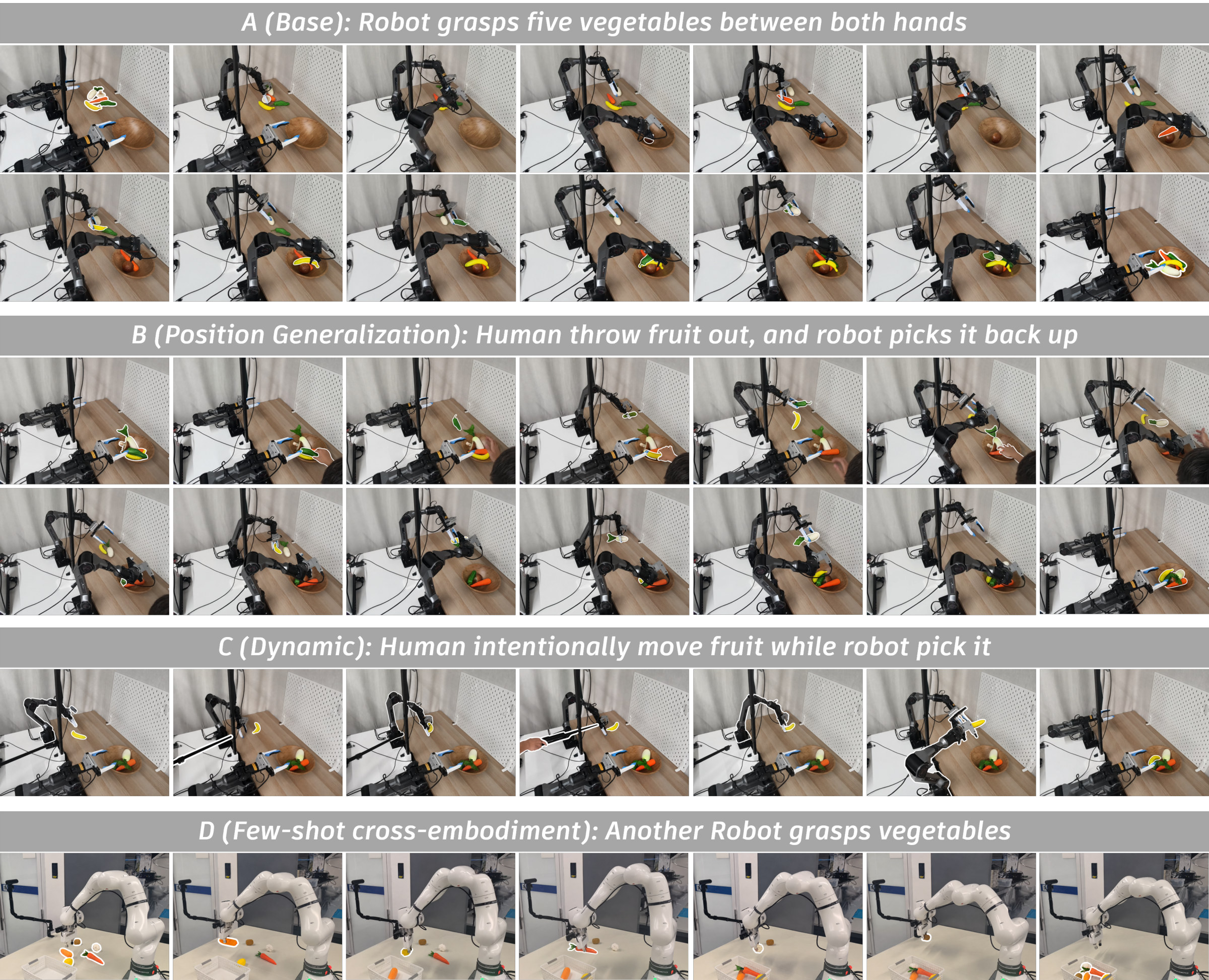
图 5:人为扰动和本体变化下的果蔬操作任务。条件 A–C 共用一个策略,该策略在 A 场景配置下采集的 100 条示范上后训练,没有 B 或 C 场景中扰动的额外示范。条件 D 评估的是另一个策略:在 A 场景采集的 100 条 Piper 示范和 D 场景采集的 10 条 Franka 示范上联合后训练。
原图注:Produce manipulation tasks under human perturbations and embodiment changes. A–C conditions share a policy post-trained on 100 demonstrations collected in the A scene configuration, with no additional demonstrations of the perturbations in B or C scene. D condition evaluates a policy jointly post-trained on 100 Piper demonstrations collected in the A scene and 10 Franka demonstrations collected in the D scene.
图 5 解读
四组关键帧序列,每组上方的灰色横条写着条件名称。A(基础)两行共 14 帧:双臂 Piper 机器人一只手从桌上抓起一个仿真蔬果(香蕉、黄瓜、胡萝卜等),在空中交给另一只手,再放进右下方的木碗,五个物体依次完成;被操作的物体用白色描边标出。B(位置泛化):碗里已经有蔬果,一个人伸手把它们拨出或扔到桌上(右侧可见人手和人头),机器人再把散落的物体逐个捡回、交接、放回碗中。C(动态):人用一根长杆拨动桌上的香蕉,使它在机器人抓取过程中移动,机器人需要追踪并抓住它。D(少样本跨本体):换成白色的单臂 Franka,把桌上的五个蔬果依次放进前方的白色篮子。从照片可以看出,A–C 都需要“抓取—交接—放置”的完整双臂序列,任务时长较长;D 则是单臂抓放,动作更简单,但训练数据里 Franka 只有 10 条示范。这张图是定性展示,帧序列都是成功案例。
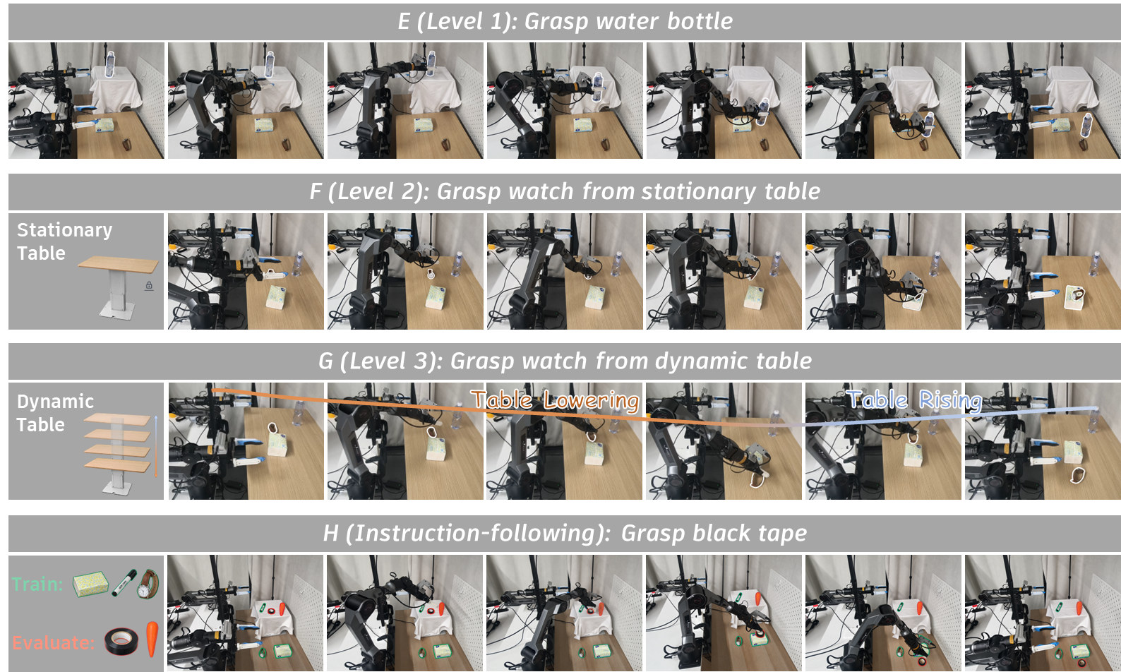
图 6:物体、桌面高度和指令目标变化下的桌面操作任务。四个条件共用一个策略,该策略在 E 场景配置下采集的 100 条示范上后训练。水瓶、纸巾盒、笔和手表包含在这些示范中,而黑色胶带和胡萝卜不在其中。
原图注:Tabletop manipulation tasks under changes in object, table height, and instruction target. All four conditions share a policy post-trained on 100 demonstrations collected in the E scene configuration. The bottle, tissue box, pen, and watch are included in these demonstrations while black tape and carrot are excluded.
图 6 解读
四行对应 E–H 四个条件。E(第 1 级):机器人从右侧铺白布的高台上抓起水瓶,放到前方木桌上。F(第 2 级):左侧小图示意一张“固定”的升降桌(带锁图标),机器人从这张高度与训练时不同的桌面上抓起手表并放下。G(第 3 级):左侧小图示意升降桌在多个高度之间移动;序列上方的橙色曲线标着“Table Lowering”(桌面下降)、蓝色曲线标着“Table Rising”(桌面上升),表示在抓取过程中桌面先降后升,机器人需要跟随目标高度的变化。H(指令跟随):左侧小图写明训练中见过的物体是纸巾盒、笔、手表(绿字 Train),评估用的是黑色胶带和胡萝卜(橙字 Evaluate);指令要求抓黑色胶带,胡萝卜是干扰物,机器人需要依照语言选对目标。E–G 的“级别”体现了难度递进:同一场景 \to 静态改变高度 \to 动态改变高度。H 同时考察“未见过的物体”和“语言选择目标”两种能力,因此它的结果难以单独归因于其中任何一种。
4.5.1真实世界任务(Real-world Tasks)
原文
We design a diverse set of challenging real-world tasks to evaluate bimanual coordination, spatial and dynamic generalization, few-shot cross-embodiment adaptation, and instruction following. The training and evaluation protocols are specified in Sec. 4.1.
译文
我们设计了一组多样且具有挑战性的真实世界任务,用于评估双臂协调、空间与动态泛化、少样本跨本体适配以及指令跟随。训练和评估协议见第 4.1 节。
解释
四类能力与图 1 雷达图的五个轴对应(分布内、位置 OOD、动态 OOD、跨本体、指令跟随)。按数值反推,雷达图的分组是:分布内 = A 与 E 的平均(SLA (94+98)/2=96),位置 OOD = B 与 F 的平均((82+84)/2=83),动态 OOD = C 与 G 的平均((76+78)/2=77),跨本体 = D(78),指令跟随 = H(80);\pi_{0.5} 的内圈数值(82、60、43、48、60)也都能这样还原。原文没有交代这一分组。
原文
For the produce tasks in Fig. 5, we post-train a single policy on 100 demonstrations of the base scene A and evaluates it in A–C. A (Base) Robot grasps five vegetables between both hands: the robot passes five objects between its arms and places them into a bowl, testing bimanual coordination. B (Position Generalization) Human throw fruit out, and robot picks it back up: we tests recovery after a person throws objects from the bowl onto the table, and the policy must retrieve them and repeat handover and placement. C (Dynamic) Human intentionally move fruit while robot pick it: we tests responsiveness to target motion during grasping, while still requiring subsequent handover and placement. D (Few-shot cross-embodiment) Another Robot grasps vegetables: To examine adaptation with limited target-robot data, we use a separate policy jointly post-trained on the 100 Piper demonstrations and 10 additional Franka demonstrations, and deploy it to a single Franka arm to place five objects into a basket.
译文
对于图 5 中的果蔬任务,我们在基础场景 A 的 100 条示范上后训练一个策略,并在 A–C 中评估。A(基础)机器人用双手传递五个蔬菜:机器人在两臂之间传递五个物体并把它们放进碗里,测试双臂协调。B(位置泛化)人把水果扔出去,机器人把它捡回来:我们测试人把物体从碗里扔到桌上之后的恢复能力,策略必须把它们取回并重复交接和放置。C(动态)人在机器人抓取时故意移动水果:我们测试抓取过程中对目标运动的响应能力,同时仍要求完成随后的交接和放置。D(少样本跨本体)另一台机器人抓取蔬菜:为考察目标机器人数据有限时的适配,我们使用另一个策略,在 100 条 Piper 示范和另外 10 条 Franka 示范上联合后训练,并将其部署到单臂 Franka 上,把五个物体放进篮子。
解释
B 的设计有一个细节:物体被扔到桌上的位置是随机的,可能落在训练示范中物体从未出现的区域,因此称为“位置泛化”。C 中物体在抓取过程中移动,要求策略在执行动作块的过程中不断根据新观测修正,这对“每次输出一个动作块、执行完再重新观测”的 \pi_{0.5} 类策略是一个挑战,结果也与执行频率、动作块长度有关,而这些参数正文没有给出。D 的 Franka 任务是“放进篮子”而非“交接后放进碗”,任务本身与 A 不同,所以它同时考察跨本体和跨任务。
原文
For the tabletop tasks in Fig. 6, we post-train one policy on 100 demonstrations collected in the E scene configuration and evaluates it across E–H. E (Level 1) Grasp water bottle: we provide a reference for basic manipulation: the robot grasps a bottle and stably places it on the destination table. F (Level 2) Grasp watch from stationary table: we test adaptation to a different static table height by transferring a watch that is already represented in the training data. G (Level 3) Grasp watch from dynamic table: we further test responsiveness to changing target height as the supporting table rises and lowers during grasping, without additional table-motion demonstrations. H (Instruction-following) Grasp black tape: Finally, we retain the E table configuration and tests instruction following with objects absent from downstream training: the robot must select and transfer black tape as instructed while ignoring a carrot distractor.
译文
对于图 6 中的桌面任务,我们在 E 场景配置下采集的 100 条示范上后训练一个策略,并在 E–H 上评估。E(第 1 级)抓水瓶:作为基本操作的参照,机器人抓起一个瓶子并稳定地放到目标桌面上。F(第 2 级)从静止的桌面上抓手表:我们通过转移一个训练数据中已出现过的手表,测试对不同静态桌面高度的适应。G(第 3 级)从移动的桌面上抓手表:我们进一步测试在抓取过程中支撑桌面升降时对目标高度变化的响应能力,没有额外的桌面运动示范。H(指令跟随)抓黑色胶带:最后,我们保持 E 的桌面配置,用下游训练中未出现过的物体测试指令跟随:机器人必须按照指令选取并转移黑色胶带,同时忽略作为干扰物的胡萝卜。
解释
F 和 G 直接考察“三维空间理解”的核心:同一个物体放在不同高度,二维图像上的外观变化不大(只有尺寸和透视的细微差异),但抓取需要的末端高度不同。如果视觉表征里有深度信息,策略就能据此调整下降高度。这是全文中与“空间对齐”假设最直接相关的一组测试。H 中的黑色胶带和胡萝卜都是下游训练没见过的物体,但胡萝卜出现在 A–D 的果蔬任务里(不同策略),且 \pi_{0.5} 的网络预训练数据中显然见过这类常见物体,因此“未见过”只是对下游 100 条示范而言。
4.5.2结果(Results)
表 11:真实世界部署比较。每种方法在每个任务上评估 50 个分别计分的物体实例,报告物体级成功率(%,\uparrow)。平均值为 A–H 的算术平均。粗体和下划线表示所列数值中的最佳和次佳。
| 方法 | A:双手传递 蔬菜 | B:抓取被人 扔出的水果 | C:抓取被人 移动的水果 | D:另一台机器人 抓取蔬菜 |
| OpenVLA-OFT(Kim et al., 2025) | 62 | 38 | 30 | 36 |
| SpatialVLA(Qu et al., 2025) | 70 | 46 | 46 | 44 |
| \pi_{0.5}(Physical Intelligence, 2025) | 74 | 52 | 42 | 48 |
| Spatial Forcing | 84 | 66 | 58 | 62 |
| SLA(本文) | 94 | 82 | 76 | 78 |
| 方法 | E:抓 水瓶 | F:从静止桌面 抓手表 | G:从移动桌面 抓手表 | H:抓未见过的 黑色胶带 | 平均 |
| OpenVLA-OFT(Kim et al., 2025) | 82 | 50 | 28 | 42 | 46.0 |
| SpatialVLA(Qu et al., 2025) | 88 | 58 | 38 | 38 | 53.5 |
| \pi_{0.5}(Physical Intelligence, 2025) | 90 | 68 | 44 | 60 | 59.8 |
| Spatial Forcing | 94 | 64 | 60 | 56 | 68.0 |
| SLA(本文) | 98 | 84 | 78 | 80 | 83.8 |
原表注:Real-world deployment comparisons. Each method is evaluated on 50 separately scored object instances per task to report the object-level success rates (%, \uparrow). Average is the arithmetic mean over A–H. Bold and underline denote the best and second-best displayed values.
表 11 解读
表分上下两块,上块是果蔬任务 A–D,下块是桌面任务 E–H,最后一列是八个条件的算术平均。五个方法中,OpenVLA-OFT 和 SpatialVLA 是外部基线(后者是带三维位置编码的 VLA),\pi_{0.5} 是 SLA 的初始化来源,SF 和 SLA 是作者团队的两个版本。平均值都能精确还原:SLA (94+82+76+78+98+84+78+80)/8=670/8=83.75,\pi_{0.5} 478/8=59.75,SF 544/8=68.0,OpenVLA-OFT 368/8=46.0,SpatialVLA 428/8=53.5。所有值都是 2 的倍数,与“每格 50 个实例”一致。SLA 在八个条件上全部第一,领先 SF 4–24 个百分点。SF 在六个条件上第二,但在 F(64 < 68)和 H(56 < 60)上不如 \pi_{0.5}。从“掉幅”看:B 相对 A,\pi_{0.5}、SF、SLA 分别掉 22、18、12;G 相对 F 分别掉 24、4、6。SLA 和 SF 在动态条件下的相对掉幅都比 \pi_{0.5} 小。统计上,每格只有 50 个实例(A、B、D 实为 10 次试验),单格标准误约 5–7 个百分点,SLA 与 SF 在 E(差 4)上的差距不显著,在其余条件(差 10–24)上大多在两个标准误以上。所有数字都来自单次评估,作者自建的任务和场景也没有公开评测协议,属于“自建场景、自己评测”的结果,可信度低于 RoboDojo 这类第三方评测。
原文
We compare OpenVLA-OFT (Kim et al., 2025), SpatialVLA (Qu et al., 2025), \pi_{0.5} (Physical Intelligence, 2025), Spatial Forcing, and SLA. Spatial Forcing applies spatial supervision only during post-training from \pi_{0.5}, whereas SLA combines spatially supervised continual pre-training with downstream post-training. As shown in Tab. 11, SLA achieves the highest success rate across all tasks while Spatial Forcing ranks second on most tasks, which supports the effectiveness of our approach. The task-specific discussion below examines several complementary capabilities of our model that are essential for real-world applications.
译文
我们比较 OpenVLA-OFT(Kim et al., 2025)、SpatialVLA(Qu et al., 2025)、\pi_{0.5}(Physical Intelligence, 2025)、Spatial Forcing 和 SLA。Spatial Forcing 只在从 \pi_{0.5} 出发的后训练中施加空间监督,而 SLA 把带空间监督的持续预训练与下游后训练结合起来。如表 11 所示,SLA 在所有任务上都取得最高成功率,Spatial Forcing 在大多数任务上排第二,这支持了我们方法的有效性。下面逐任务的讨论考察了我们模型在真实应用中不可或缺的几种互补能力。
解释
“大多数任务排第二”具体是 8 个中的 6 个(A、B、C、D、E、G)。下面八段逐一讨论,数字都与表 11 一致,解释框只补充文字没有提到的地方。
原文
A: Bimanual coordination. The success rates are 74% for \pi_{0.5}, 84% for Spatial Forcing, and 94% for SLA, corresponding to gains of 10 and 20 percentage points over the base policy. These gains support the value of spatial supervision for the complete grasp–handover–placement sequence, with the full SLA recipe providing an additional benefit over post-training-only Spatial Forcing.B: Recovery from positional changes. The success rates increase from 52% with \pi_{0.5} to 66% with Spatial Forcing and 82% with SLA. Relative to A, the corresponding reductions are 22, 18, and 12 points. A smaller reduction for SLA indicates more robust reuse of the learned manipulation skill after object relocation. Because A and B share a trained policy, this comparison concerns generalization to the intervention rather than fitting additional recovery demonstrations.
译文
A:双臂协调。\pi_{0.5}、Spatial Forcing 和 SLA 的成功率分别为 74%、84% 和 94%,相对基础策略分别提高 10 和 20 个百分点。这些提升支持了空间监督对完整的“抓取—交接—放置”序列的价值,完整的 SLA 配方相对只在后训练中对齐的 Spatial Forcing 还带来了额外收益。B:位置变化后的恢复。成功率从 \pi_{0.5} 的 52% 提高到 Spatial Forcing 的 66% 和 SLA 的 82%。相对于 A,对应的下降分别为 22、18 和 12 个百分点。SLA 下降更少,说明物体被挪动后它能更稳健地复用学到的操作技能。由于 A 和 B 共用一个训练好的策略,这一比较涉及的是对干预的泛化,而不是拟合额外的恢复示范。
解释
A 是分布内条件,SLA 的 94% 已接近上限。B 的“下降量”是一个比绝对值更有信息量的指标:它刻画了同一策略从训练条件到扰动条件损失了多少。不过 B 的物体位置是由人随手扔出决定的,不同方法面对的位置分布并不完全相同,正文没有说明如何控制这一变量。
原文
C: Response to moving targets. The success rates are 42%, 58%, and 76% for \pi_{0.5}, Spatial Forcing, and SLA, respectively, placing SLA 18 points above Spatial Forcing. This advantage is consistent with more effective use of current visual observations when the target moves during grasping, while retaining the ability to finish the subsequent handover and placement.D: Adaptation with limited target-embodiment data. Under the training budget of 100 Piper and 10 Franka demonstrations, the success rates are 48% for \pi_{0.5}, 62% for Spatial Forcing, and 78% for SLA. Such a result supports the usefulness of spatial supervision when adapting manipulation across embodiments with limited target domain data. The 16-point margin over Spatial Forcing further favors the complete SLA recipe in this joint-training setting.
译文
C:对移动目标的响应。\pi_{0.5}、Spatial Forcing 和 SLA 的成功率分别为 42%、58% 和 76%,SLA 比 Spatial Forcing 高 18 个百分点。这一优势与“目标在抓取过程中移动时能更有效地利用当前视觉观测,同时保留完成后续交接和放置的能力”相一致。D:目标本体数据有限时的适配。在 100 条 Piper 和 10 条 Franka 示范的训练预算下,\pi_{0.5}、Spatial Forcing 和 SLA 的成功率分别为 48%、62% 和 78%。这一结果支持了在目标域数据有限时,空间监督对跨本体适配操作的作用。比 Spatial Forcing 高 16 个百分点,进一步支持完整的 SLA 配方在这种联合训练设定下的优势。
解释
C 的解释(“更有效地利用当前视觉观测”)与状态丢弃的设计动机相合,但没有直接证据区分是空间对齐、持续预训练还是状态丢弃起的作用。D 是持续预训练最可能发挥作用的条件:持续预训练语料中有 DROID 和 MolmoAct 两个 Franka 数据集,SLA 在后训练前就已见过大量 Franka 数据,而 SF 直接从 \pi_{0.5} 出发(\pi_{0.5} 的预训练数据中也含 Franka,但未经本文的统一动作表示)。因此 D 上 16 个百分点的优势,更像是“持续预训练见过目标本体”的收益,而不一定来自空间对齐。
原文
E: Execution in the training scene configuration. The success rates of 90%, 94%, and 98% means that both \pi_{0.5} and our policies are near the upper end of the metric. The 4-point margin between SLA and Spatial Forcing corresponds to two additional successful object instances out of 50. Such closely spaced values would establish basic manipulation competence while leaving limited headroom for improvement, making the changed conditions in F–H more informative about generalization.F: Adaptation to a different table height. The success rates of Spatial Forcing is 64%, below the 68% of \pi_{0.5}, while SLA reaches 84%. This result indicates that the benefits of post-training-only spatial supervision are not uniform across conditions. The 20-point margin over Spatial Forcing favors the complete recipe under the table height changes.
译文
E:在训练场景配置中执行。90%、94% 和 98% 的成功率意味着 \pi_{0.5} 和我们的策略都接近该指标的上限。SLA 与 Spatial Forcing 之间 4 个百分点的差距,相当于 50 个物体实例中多成功 2 个。如此接近的数值确立了基本的操作能力,但留下的提升空间有限,因此 F–H 中改变后的条件对于泛化更有参考价值。F:适应不同的桌面高度。Spatial Forcing 的成功率为 64%,低于 \pi_{0.5} 的 68%,而 SLA 达到 84%。这一结果表明,只在后训练中做空间监督的收益并不是在各种条件下都一致的。比 Spatial Forcing 高 20 个百分点,支持完整配方在桌面高度变化下的优势。
解释
E 一段的自我限定是诚实的:4 个百分点只是 2 个实例,不应过度解读。F 是一个有意思的结果:SF 的空间对齐在“桌面高度改变”这一最直接的三维泛化测试中反而不如不对齐的 \pi_{0.5}。作者只说“收益不一致”,没有分析原因;这也提醒读者,后训练阶段只用 100 条同一高度的示范做对齐,三维表征可能被拟合到训练高度上,而持续预训练中见过的大量不同场景高度可能才是 SLA 在 F 上表现好的关键。
原文
G: Manipulation during table motion. The success rates are 44% for \pi_{0.5}, 60% for Spatial Forcing, and 78% for SLA. Compared with F, the reductions are 24, 4, and 6 points, respectively. The result means that both spatially supervised policies retain more abilities of their static-condition performance, while SLA maintains the highest absolute success rate. This pattern supports spatial supervision under changing geometry and the additional benefit of the full recipe, suggesting that our methods has the powerful static-to-dynamic fitness.H: Instruction-guided manipulation of an unseen object. The success rates are 60% for \pi_{0.5}, 56% for Spatial Forcing, and 80% for SLA. A 24-point gain over Spatial Forcing supports the ability to follow the specified target while transferring grasp-and-place behavior to an object excluded from downstream training. This comparison attributes the gains of our method to language-following and geometric reasoning abilities.
译文
G:桌面运动中的操作。\pi_{0.5}、Spatial Forcing 和 SLA 的成功率分别为 44%、60% 和 78%。与 F 相比,下降分别为 24、4 和 6 个百分点。这一结果意味着两种带空间监督的策略都更多地保留了其静态条件下的能力,而 SLA 保持了最高的绝对成功率。这一模式支持了在几何变化下进行空间监督的作用以及完整配方的额外收益,表明我们的方法具有很强的从静态到动态的适应能力。H:对未见物体的指令引导操作。\pi_{0.5}、Spatial Forcing 和 SLA 的成功率分别为 60%、56% 和 80%。比 Spatial Forcing 高 24 个百分点,支持了在把抓放行为迁移到下游训练中未出现的物体时,仍能遵循指定目标的能力。这一比较把我们方法的收益归因于语言跟随和几何推理能力。
解释
G 的“下降量”比较中,SF(4)其实比 SLA(6)掉得更少,作者对此的表述是“两种带空间监督的策略都保留了更多能力”,措辞准确。H 的最后一句“把收益归因于语言跟随和几何推理能力”是全文中最强、证据最弱的断言之一:H 只有一个任务、一组物体、50 次试验,而且 SF 在这里比 \pi_{0.5} 还低 4 个百分点,说明“空间对齐”本身并不提升指令跟随;SLA 的优势更可能来自持续预训练中大量多样任务带来的语义与物体泛化。另外,LIBERO-Plus 的语言维度上 SLA(83.5)低于 SF(85.6),与这里的结论方向相反。
原文
Taken together, these results supports the significance of our SLA training approach across spatial perturbations, embodiment adaptation, and language-guided object manipulation. our SLA supervision uses auxiliary components only during training, retaining the original policy backbone and action-generation architecture for deployment. This compatibility enables continued training without adding policy computation at inference.
译文
综合来看,这些结果支持了 SLA 训练方法在空间扰动、本体适配和语言引导的物体操作中的重要性。我们的 SLA 监督只在训练中使用辅助组件,部署时保留原有的策略主干和动作生成架构。这种兼容性使得持续训练成为可能,而不会在推理时增加策略的计算量。
解释
这一总结段落重复了“推理零开销”的卖点。就八个真机部署条件而言,正文没有提到使用记忆机制,这一点应当成立;但如表 5 解读所述,RoboDojo-Real 上的 SLA 加入了推理时也要保留的历史图像输入。
5结论(Conclusion)
原文
In this work, we presented SLA, a Spatial-Language-Action Model that develops transferable spatial understanding through continual pre-training and downstream post-training. By aligning intermediate visual representations with a frozen 3D perception model, our approach integrates geometric supervision into action learning while directly reusing pretrained VLA weights. A unified robot-data corpus and adaptive layer selection support training across heterogeneous embodiments and scenes, while available depth and calibration annotations enrich the spatial supervision. The teacher and alignment modules are required only during training.
译文
在本工作中,我们提出了 SLA,一个通过持续预训练和下游后训练发展可迁移空间理解的空间—语言—动作模型。通过把中间层视觉表征与冻结的三维感知模型对齐,我们的方法把几何监督融入动作学习,同时直接复用预训练 VLA 的权重。统一的机器人数据语料库和自适应层选择支持了在异构本体和场景上的训练,而可得的深度和标定标注丰富了空间监督。教师模型和对齐模块只在训练时需要。
解释
结论第一段重述方法,没有新信息。值得留意的是用词:“transferable spatial understanding”(可迁移的空间理解)是全文的核心主张,但本文对“空间理解”的直接度量只有图 2 的定性深度探测(而且是在 OpenVLA-OFT 上做的),对“可迁移”的度量则是下游成功率。没有对 SLA 本身的视觉表征做定量的深度或三维结构探测,也没有比较持续预训练前后表征的变化。
原文
Extensive evaluations demonstrate state-of-the-art performance on RoboDojo-Real, RoboTwin 2.0 under the Clean2Random setting, RoboCasa-Panda, and LIBERO-Plus, alongside improved spatial and dynamic generalization, downstream data efficiency, and few-shot cross-embodiment adaptation. Controlled experiments further show that applying spatial alignment during both training stages consistently outperforms either single-stage alternative across the tested data scales. These findings support developing spatial understanding during continual pre-training and reinforcing it during downstream adaptation, offering a practical path toward spatially informed robotic foundation models.
译文
大量评估表明,SLA 在 RoboDojo-Real、Clean2Random 设定下的 RoboTwin 2.0、RoboCasa-Panda 和 LIBERO-Plus 上取得了最先进的性能,并在空间与动态泛化、下游数据效率和少样本跨本体适配方面有所提升。受控实验进一步表明,在两个训练阶段都施加空间对齐,在所测试的各个数据规模下都始终优于只在单一阶段对齐的两种做法。这些发现支持在持续预训练中发展空间理解、并在下游适配中加以强化,为构建具备空间信息的机器人基础模型提供了一条切实可行的路径。
解释
回顾全文证据,可以把结论分成三个强度等级。证据较强:表 6 的 2\times2 消融表明,在同一批持续预训练数据上,加对齐损失与否差别很大(100% 数据时 63.2 对 48.2),两阶段对齐的收益近似可加;真机八个条件上 SLA 对 SF 的一致领先(4–24 个百分点)。证据中等:RoboTwin Clean2Random 上的大幅领先,但它依赖于对状态丢弃概率极为敏感的后训练配置(表 8)。证据较弱:LIBERO-Plus(领先 0.3)、RoboCasa-Panda(领先 0.8)和 RoboDojo-Real(领先 2.2,且叠加了记忆机制)上的“最先进”,差距都在噪声或混杂因素范围内。结论段没有讨论局限性。从正文可以归纳出几项:训练成本高(每次持续预训练约 5,000 GPU 小时,外加教师模型前向);关键超参数(\alpha、持续预训练的状态丢弃概率、数据混合比例)未给出;消融大多只在 RoboTwin 一个仿真基准上做、单次运行;真机评测为自建场景且样本量小。
附录概览(Appendix Overview)
解释
本部分的处理方式。按照本工作区的翻译范围约定,正文到结论为止逐段翻译和解释;附录不再逐段对照,而是用中文段落概述其内容,并挑选三张有代表性的附录表格(表 13、14、15)重排后加以解读。表编号沿用原文(原文附录没有重置表计数器,表 12 和表 16 两张逐任务长表只在文字中概述)。附录原文请见 arXiv 原文第 27–31 页。
A 补充结果(Additional Results)
原文附录 A 给出四个基准的逐任务结果,目的是展示 SLA 在不同任务上的强项和短板。A.1(表 12)列出 RoboTwin 2.0 全部 50 个任务在 Clean2Clean 和 Clean2Random 下的成功率,每个设定每任务 100 次试验。逐任务平均为 85.96 和 72.34,与正文表 3 的 86.0、72.3 一致。有 10 个任务的 Clean2Clean 达到 100%,其中 Grab Roller 和 Shake Bottle 在两种设定下都是 100%。随机化带来的掉幅高度依赖任务:Place Cans Plasticbox 从 96 掉到 40,Handover Block 从 91 掉到 38,Pick Dual Bottles 从 97 掉到 55;而 Turn Switch(61 \to 62)和 Move Stapler Pad(33 \to 41)反而在随机场景中略高。Clean2Random 最低的是 Stack Blocks Three(27)和 Hanging Mug(31),都是需要精细对准或多步堆叠的任务。作者据此指出“干净条件下表现好并不总能转化为随机化条件下同样可靠的执行”。A.2(表 13)和 A.3(表 14)分别是 RoboCasa-Panda 和 RoboDojo-Real 的逐任务结果,下面重排并解读。表 13:SLA 在 RoboCasa-Panda 上的逐任务成功率(%,\uparrow)。每个数值是三个评估种子(195、196、197)上的算术平均,每个任务每个种子 50 次试验(每任务 150 次,共 3,600 次)。任务按评估协议顺序排列,左侧为任务 1–12,右侧为 13–24。
| 任务 | 平均 SR(%) | 任务 | 平均 SR(%) |
| PnPCounterToCab | 54.7 | OpenDrawer | 84.0 |
| PnPCabToCounter | 21.3 | CloseDrawer | 97.3 |
| PnPCounterToSink | 68.0 | TurnOnStove | 49.3 |
| PnPSinkToCounter | 58.0 | TurnOffStove | 22.7 |
| PnPCounterToMicrowave | 41.3 | TurnOnSinkFaucet | 72.0 |
| PnPMicrowaveToCounter | 34.7 | TurnOffSinkFaucet | 94.0 |
| PnPCounterToStove | 75.3 | TurnSinkSpout | 82.0 |
| PnPStoveToCounter | 67.3 | CoffeeSetupMug | 25.3 |
| OpenSingleDoor | 77.3 | CoffeeServeMug | 61.3 |
| CloseSingleDoor | 92.0 | CoffeePressButton | 85.3 |
| OpenDoubleDoor | 95.3 | TurnOnMicrowave | 93.3 |
| CloseDoubleDoor | 90.0 | TurnOffMicrowave | 100.0 |
| 24 个任务的平均 | 68.4 | ||
原表注:Per-task success rates of SLA on RoboCasa-Panda (%, \uparrow). Each value is the arithmetic mean over three evaluation seeds (195, 196, and 197), with 50 trials per task and seed (150 trials per task; 3,600 trials in total). Tasks follow the evaluation-protocol order, with tasks 1–12 on the left and 13–24 on the right.
表 13 解读
任务名的前缀说明了类型:PnP(pick and place,抓放,从 A 处拿到 B 处)、Open/Close(开关柜门、抽屉)、TurnOn/TurnOff(操作炉灶、水龙头、微波炉)、Coffee(咖啡机相关)。24 项求和为 1641.7,除以 24 得 68.40,与正文一致;成功率超过 80% 的恰好 10 项,与正文第 4.3.3 节的说法一致。规律很明显:铰接物体和按钮类任务(开关门、抽屉、微波炉、水龙头)普遍在 80–100%;抓放类任务普遍较低,尤其是“从柜子/微波炉里拿出来”(PnPCabToCounter 21.3、PnPMicrowaveToCounter 34.7)比“放进去”更难,可能是因为在狭窄空间里抓取需要更准确的深度判断;TurnOffStove(22.7)和 CoffeeSetupMug(25.3)也很低,前者需要精确定位小旋钮,后者需要把杯子准确放到咖啡机出水口下。附录正文只挑了表现好的任务来讲(CloseDrawer、OpenDoubleDoor、TurnOnMicrowave),没有讨论这些弱项,而这些弱项恰恰是“精细空间定位”类任务,与本文要提升的能力最相关。
表 14:SLA 在 RoboDojo 真实世界基准上的逐任务结果。得分(\uparrow)缩放到 0–100,SR(%,\uparrow)衡量任务完成。均值在每种本体的六个任务内等权,总体平均对三种本体等权。
| 本体 | 任务 | 得分 | SR(%) |
| ARX X5 | cover_blocks | 65.0 | 50 |
| store_in_safe | 100.0 | 100 | |
| pack_and_pour_fruit | 70.0 | 40 | |
| make_bread | 0.0 | 0 | |
| make_food | 29.0 | 20 | |
| insert_tubes | 40.0 | 20 | |
| 均值 | 50.7 | 38.3 | |
| Piper | stand_up_bottles | 95.0 | 90 |
| stack_bowls | 90.0 | 90 | |
| stack_and_cover_blocks | 30.0 | 10 | |
| insert_charger | 5.0 | 0 | |
| fill_pen_holder | 72.0 | 60 | |
| put_objects_into_basket | 70.0 | 70 | |
| 均值 | 60.3 | 53.3 | |
| Piper X | sweep_blocks | 0.0 | 0 |
| disassemble_LEGO | 0.0 | 0 | |
| classify_objects | 48.0 | 40 | |
| hang_mugs | 8.0 | 0 | |
| cap_pen | 18.0 | 0 | |
| pack_objects_into_backpack | 22.0 | 20 | |
| 均值 | 16.0 | 10.0 | |
| 总体平均 | 42.3 | 33.9 | |
原表注:Per-task results of SLA on the RoboDojo real-world benchmark. Score (\uparrow) is scaled to 0–100, and SR (%, \uparrow) measures task completion. Means give equal weight to the six tasks within each embodiment; the overall average gives equal weight to the three embodiments.
表 14 解读
每种本体六个任务,每个任务的 SR 都是 10 的倍数,说明每任务 10 次试验,这与表 5 中本体级 SR 为 1/60 的倍数相符。18 个任务里有 6 个完全失败(SR 为 0),Piper X 上六个任务中四个为 0,只有 classify_objects(40%)和 pack_objects_into_backpack(20%)有成功。插入类任务(insert_charger、insert_tubes)和精细装配(disassemble_LEGO、cap_pen)普遍很差。本表与正文表 5 不一致。按本表各本体的均值是:ARX X5 得分 50.7、SR 38.3;Piper 得分 60.3、SR 53.3;Piper X 得分 16.0、SR 10.0。而表 5 中 SLA 一行是 ARX X5 50.3/36.7、Piper 60.3/55.0、Piper X 16.3/10.0。逐项相加可以验证本表的均值是由六个任务正确平均得到的(如 ARX SR (50+100+40+0+20+20)/6=38.3)。两张表的三本体总平均碰巧都是 42.3 和 33.9(本表 (50.7+60.3+16.0)/3=42.3、(38.3+53.3+10.0)/3=33.9;表 5 (50.3+60.3+16.3)/3=42.3、(36.7+55.0+10.0)/3=33.9),但各本体的数字对不上,ARX X5 与 Piper 的 SR 差异各约 1.7 个百分点(相当于一次试验)。原文未解释,可能是两张表取自不同的评测轮次或抄录错误。
表 15:五个能力维度上的 RoboDojo 仿真基准结果。得分(\uparrow)反映部分任务进度,SR(%,\uparrow)衡量二元的任务完成。对比方法的结果取自官方排行榜(Chen et al., 2026b),SLA 在本地评估。逐任务结果见表 16。粗体和下划线表示所列数值中的最佳和次佳。
| 方法 | 泛化 | 精度 | 长时程 | 记忆 | 开放 | 平均 | ||||||
| 得分 | SR | 得分 | SR | 得分 | SR | 得分 | SR | 得分 | SR | 得分 | SR | |
| InternVLA-A1.5(Cai et al., 2026a) | 10.4 | 6.8 | 15.2 | 10.2 | 23.8 | 13.8 | 4.9 | 3.6 | 1.4 | 1.4 | 11.2 | 7.1 |
| \pi_{0.5}(Physical Intelligence, 2025) | 13.4 | 8.2 | 12.4 | 5.5 | 23.5 | 14.7 | 5.9 | 4.7 | 2.0 | 1.7 | 11.4 | 6.9 |
| SimpleMemVLA(Yin et al., 2026) | 6.4 | 4.0 | 7.4 | 2.9 | 14.6 | 5.5 | 33.7 | 33.2 | 0.9 | 0.8 | 12.6 | 9.3 |
| KinRT(Yang et al., 2026b) | 14.0 | 8.6 | 15.7 | 9.9 | 26.4 | 18.1 | 4.8 | 3.6 | 4.2 | 3.8 | 13.0 | 8.8 |
| CogWAM(Wang et al., 2026d) | 12.8 | 9.3 | 20.5 | 14.6 | 27.4 | 18.2 | 8.2 | 7.0 | 2.9 | 2.7 | 14.3 | 10.3 |
| EWAM(Wang et al., 2026b) | 15.1 | 9.7 | 22.2 | 12.3 | 30.2 | 18.1 | 7.4 | 6.0 | 1.1 | 0.8 | 15.2 | 9.4 |
| Spatial Forcing | 14.1 | 9.3 | 17.3 | 10.6 | 23.3 | 14.6 | 5.4 | 4.1 | 1.8 | 1.6 | 12.4 | 8.0 |
| SLA(本文) | 15.3 | 9.4 | 16.0 | 11.2 | 22.3 | 11.9 | 26.2 | 25.8 | 2.0 | 1.9 | 16.4 | 12.0 |
原表注:RoboDojo simulation benchmark results across five capability dimensions. Score (\uparrow) captures partial task progress, and SR (%, \uparrow) measures binary task completion. Results of the compared methods are taken from the official leaderboard (Chen et al., 2026b), and SLA is evaluated locally. Per-task results are shown in Tab. 16. Bold and underline denote the best and second-best displayed values.
表 15 解读
五组列对应五个能力维度,每组有得分和 SR;最后是五个维度的等权平均。SLA 的平均 (15.3+16.0+22.3+26.2+2.0)/5=16.4、SR (9.4+11.2+11.9+25.8+1.9)/5=12.0,均为表中最高;比 \pi_{0.5} 高 5.0 分和 5.1 个百分点,与附录文字一致。但拆开看,SLA 的领先几乎全部来自“记忆”维度:SLA 在记忆上得 26.2/25.8,而 SF 只有 5.4/4.1,\pi_{0.5} 只有 5.9/4.7,只有专门做记忆的 SimpleMemVLA 更高。SLA 加了记忆机制,SF 和 \pi_{0.5} 显然没有。如果去掉记忆维度,只看其余四个维度的平均得分,SLA 为 (15.3+16.0+22.3+2.0)/4=13.9,低于 EWAM 的 17.2、CogWAM 的 15.9 和 KinRT 的 15.1,也略低于 SF 的 14.1。SLA 在长时程(22.3/11.9)上甚至低于 \pi_{0.5}(23.5/14.7)和 SF(23.3/14.6)。因此这张表能支持的结论是“记忆机制在 RoboDojo 的记忆类任务上很有效”,而不是“空间对齐的持续预训练在仿真上全面领先”。另外,对比方法取自官方排行榜,SLA 是本地评测,评测环境可能不完全一致。
B 记忆机制(Memory Mechanism)
附录 B 说明了 RoboDojo-Real(以及 RoboDojo-Sim)后训练中使用的记忆机制。与一些用专门记忆模块的 VLA 不同,这里的做法非常朴素:把主相机过去的若干帧当作额外的图像输入,与当前视角一起送进同一个视觉—语言主干。记忆的构造(式 11)。设 I_k 为当前回合主相机的第 k 帧(k=0 为回合第一帧),f 为该本体的录制频率(Piper X 为 25 Hz,ARX X5 和 Piper 为 30 Hz)。在第 t 帧生成动作块时,记忆上下文由 9 帧组成:\mathcal M_t=[I_0, I_{\max(t-8f,0)}, I_{\max(t-7f,0)},\ldots,I_{\max(t-f,0)}],即回合初始帧,加上过去 8 秒中每秒一帧,按从旧到新排列。初始帧记录了操作开始前的场景布局,全程可用;最近的帧刻画短期进展和单帧无法体现的运动。回合开始后的前 8 秒内,缺失的历史帧用初始帧填补。记忆帧只取自主相机,腕部相机只提供当前帧。记忆的编码。每个记忆帧缩放到与当前视角相同的分辨率,由同一个 SigLIP 编码器编码为 256 个视觉 token。前缀中图像 token 按时间顺序排列:初始帧、从旧到新的近期帧、三个当前视角,之后是语言 token;顺序只由 token 位置体现,没有额外的时间嵌入。记忆 token 与其他前缀 token 之间是全注意力,动作专家也能访问它们。记忆帧不参与空间对齐:既不送入 OmniVGGT,对齐损失式 (5) 也只在当前视角的 token 上计算。训练与推理。后训练时,数据加载器按式 (11) 为每个样本取出记忆帧。部署时,一个在线缓冲区以相机频率记录主相机帧(包括不请求新动作块的控制步),保留初始帧和最近 8 秒的帧;每次请求新动作块时,按式 (11) 组装 \mathcal M_t,使推理时看到的记忆与训练时一致。每个回合开始时清空缓冲区,防止跨回合泄漏。解释
代价估算。9 个记忆帧 \times 256 token =2{,}304 个额外视觉 token,而三个当前视角只有 768 个,视觉前缀长度变为原来的 4 倍。由于注意力的计算量随序列长度平方增长,前缀部分的计算和显存开销会显著上升。这与正文反复强调的“推理架构和开销与 \pi_{0.5} 相同”形成对照:在 RoboDojo 两个基准上,部署的模型并不是“零额外开销”的。表 15 也说明,这一机制本身(而非空间对齐)是 SLA 在 RoboDojo-Sim 上领先的主要来源;正文表 5 没有给出“不加记忆”的 SLA 结果,因此无法判断 RoboDojo-Real 上的领先中有多少来自记忆。
译者附注:原文数字核对与阅读提示汇总
以下各条已在正文对应位置的解释框中说明,这里集中列出。总体而言,正文中的引用数字与表格是自洽的:表 1 三列合计、表 2–4 与文字中的差值、表 3/7/8/9/10 各行的平均值、表 6 中的各项差值、表 11 八个条件的平均(如 670/8=83.75),以及附录表 12、13 的逐任务平均都能精确还原。问题主要集中在三处:附录逐任务表与正文表 5 对不上,图 4 的起点画法掩盖了与 Spatial Forcing 结果的矛盾,以及若干影响公平比较的设置没有交代(状态丢弃、记忆机制、超参数)。| 位置 | 说明 |
| 表 5 / 表 14 | SLA 的各本体数字不一致。表 14 由六个任务平均得到 ARX X5 50.7/38.3、Piper 60.3/53.3、Piper X 16.0/10.0(可逐项验算);表 5 却写 ARX X5 50.3/36.7、Piper 60.3/55.0、Piper X 16.3/10.0。两表三本体总平均都是 42.3/33.9,但各本体对不上,原文未解释。 |
| 表 6 / 图 4 / 表 3 | 图注称“所有曲线从共同的 \pi_{0.5} 基线出发”(0% 处均为 46.0)。但“只后训练对齐、0% 持续预训练”就是 Spatial Forcing,表 3 中其 Clean2Random 为 62.6。按表 6,“只后训练对齐”在 5%–100% 数据下为 45.6–57.1,全部低于不做持续预训练的 SF;“都不对齐”在 5% 时(43.8)也低于 \pi_{0.5}。即不加对齐的持续预训练对后续适配有害或无益,原文未讨论,且图的画法掩盖了这一点。 |
| 表 8 | 同一持续预训练检查点,后训练状态丢弃 0%/25%/50%/75%/100% 的平均 SR 为 38.1/79.2/53.9/61.9/56.7,极不平滑。0% 时远低于 \pi_{0.5}(58.3)和 SF(68.7)。正文未说明 \pi_{0.5}、SF 等基线是否使用状态丢弃,也未给出持续预训练阶段的丢弃概率。主结果 79.2 恰是这条非单调曲线的最高点。 |
| 表 5 / 附录 B | RoboDojo-Real(及 RoboDojo-Sim)上的 SLA 额外使用了记忆机制(9 帧历史主相机图像,视觉前缀 token 数变为 4 倍),推理时保留。摘要、引言、结论所称“保持原推理架构、无额外开销”在这两个基准上不成立。表 5 没有“无记忆”的 SLA,也没有 SF 行,无法分离各因素的贡献。 |
| 表 15(附录) | RoboDojo-Sim 的领先几乎全部来自记忆维度(SLA 26.2/25.8,SF 5.4/4.1)。去掉记忆维度,SLA 其余四维平均得分 13.9,低于 EWAM(17.2)、CogWAM(15.9)、KinRT(15.1)和 SF(14.1);长时程维度还低于 \pi_{0.5}。此基准上空间对齐只用于持续预训练。 |
| 第 3.1 节 / 图 2 | 深度探测用的是 OpenVLA-OFT(Kim et al., 2025),不是 SLA 所基于的 \pi_{0.5};“对齐后”的嵌入来自哪个模型、什么数据未交代。文中称“linear probing”,实际训练的是 DPT 头(非线性)。称可“量化”空间信息,但只给了 4 组定性深度图,无数值指标。 |
| 第 3.2 节 | 对齐权重 \alpha 的取值、位置嵌入 E 的形式、教师特征维度均未给出;无 \alpha 消融。门控在各层之间无归一化,未给出学到的门控权重分析,也缺少“各层等权平均”的对照。 |
| 第 3.3 节 / 表 1 | 表 1 的 170 万回合、14,330 小时是处理前的源数据规模;InternData-A1 只保留 3%–10%,RoboCasa365 MimicGen 只保留 0.5%,处理后实际规模未给出。仿真数据(InternData-A1、RoboCasa365)占源回合数约 74%。各数据集混合比例未给出。 |
| 第 3.3.1 节 / 表 4 | 持续预训练语料含 RoboCasa365 预训练子集,与下游 RoboCasa-Panda 同平台(场景、资产、Panda 机械臂)。“只用 50 条示范超过用 300–3,000 条的方法”部分来自这层领域重叠;对同样 50 条示范的 SF 只领先 0.8,对 Cosmos Policy 领先 1.3,均在约 0.77 个百分点标准误的一到两倍内。 |
| 表 2 | SLA 对第二名 Qwen-RobotManip 只领先 0.3(标准误约 0.34)。七个维度中机器人、语言、布局三项不如 SF(73.8 对 79.3、83.5 对 85.6、86.2 对 88.3);正文只与 \pi_{0.5} 比较“七维全部提升”,其中机器人维度仅 +0.2。 |
| 表 7、9、10 | 未说明固定层、旋转表示、教师模型这些变体是否重做了持续预训练。第 4.4.4 节说明旋转表示只在后训练中更换,因此比较的是“在旋转向量上预训练后换表示微调”的代价。表 10 用的是“自采的 RoboTwin 干净数据”(最好只有 46.0%),与其他表不可横比;表中 VGGT 行(42.5)与无标定 OmniVGGT(42.8)几乎相同,正文未提及。 |
| 表 11 | 物体级 SR 中 A、B、D 为 10 次试验 \times 5 个物体,实例间相关,有效样本量约 10;单格标准误约 5–7 个百分点,E 上 SLA 与 SF 的差距(4)不显著。均为单次评估的自建场景。H 的结论“归因于语言跟随和几何推理”证据薄弱(单任务,且 SF 低于 \pi_{0.5};LIBERO-Plus 语言维度 SLA 低于 SF)。D 上的优势可能主要来自持续预训练语料中大量 Franka 数据(DROID、MolmoAct)。 |
| 图 1 | 柱状图中 RoboDojo-Real 的 42.3 对 38.9 是“得分”,而摘要和引言引用的是成功率 33.9%;雷达图五个维度由表 11 的条件两两平均得到(分布内 = A,E;位置 OOD = B,F;动态 OOD = C,G;跨本体 = D;指令跟随 = H),原文未说明分组。 |
| 第 4.2 节 | 未说明基线(\pi_{0.5}、SF、OpenVLA-OFT、SpatialVLA)的后训练步数、批大小是否与 SLA 相同;数据扩展消融中各数据比例的持续预训练步数是否相同也未说明。动作块长度、执行频率未给出。 |
| 措辞与笔误 | 引言 “has propose a implicit … to enbow”“still concentrate”“we combines”“down-streaming”“stengthen”;第 4.1 节 “plenty real-world deployments”“successs”;第 4.5 节多处主谓不一致(“we tests”“evaluates”“these results supports”“our methods has”);图 3 源文件名拼作 “rotataion”。译文已按原意改正。 |