ODE 策略:通过学习动作动态
而非动作本身来进行机器人学习
ODE Policy: Robot Learning via Action Dynamics, Not Actions
Jindou Jia^{*\ddagger}, Jingliang Li^{*}, Kuangji Zuo^{*}, Tuo An^{*}, Yuxuan Hu, Mengfei Zhao, Bofan Lyu,
Jiaqi Bai, Daoyuan Zhu, Hengyu Dai, Junpeng Zhang, Jianfei Yang^{\dagger}
MARS Lab,南洋理工大学
^*共同第一作者 ^\ddagger项目负责人 ^\dagger通讯作者
arXiv:2611.01729v1 [cs.RO],2026 年 11 月 1 日提交(35 页,23 幅图)
项目主页:https://ntumars.github.io/ODE/ 代码:https://github.com/NTUMARS/ODE-POLICY
中文逐段翻译与解释
整理日期:2026 年 11 月 4 日
而非动作本身来进行机器人学习
ODE Policy: Robot Learning via Action Dynamics, Not Actions
Jindou Jia^{*\ddagger}, Jingliang Li^{*}, Kuangji Zuo^{*}, Tuo An^{*}, Yuxuan Hu, Mengfei Zhao, Bofan Lyu,
Jiaqi Bai, Daoyuan Zhu, Hengyu Dai, Junpeng Zhang, Jianfei Yang^{\dagger}
MARS Lab,南洋理工大学
^*共同第一作者 ^\ddagger项目负责人 ^\dagger通讯作者
arXiv:2611.01729v1 [cs.RO],2026 年 11 月 1 日提交(35 页,23 幅图)
项目主页:https://ntumars.github.io/ODE/ 代码:https://github.com/NTUMARS/ODE-POLICY
中文逐段翻译与解释
整理日期:2026 年 11 月 4 日
解释
阅读方式。沿用本工作区已完成译文的三联框:灰色框保留英文原文,蓝色框给出中文译文,橙色框解释概念、公式、设计动机和结论边界。图片使用原论文源码中的矢量图,表格完整重排,均附原注、译注和绿色解读框;两个伪代码算法以中文重排。保留原章节、公式和图表编号(附录图表带前缀 S);正文引用沿用原文的“作者,年份”格式,参考文献列表从略。解释框是本译稿的分析,不属于作者原文。
来源与许可。原论文:https://arxiv.org/abs/2611.01729v1;PDF:https://arxiv.org/pdf/2611.01729v1。本文以 arXiv 默认的非独占分发许可(arXiv.org perpetual, non-exclusive license)发布,不是知识共享许可;本译稿仅供个人学习研究,不宜公开再分发。英文内容以下载的 v1 源码及 PDF 为依据。
来源与许可。原论文:https://arxiv.org/abs/2611.01729v1;PDF:https://arxiv.org/pdf/2611.01729v1。本文以 arXiv 默认的非独占分发许可(arXiv.org perpetual, non-exclusive license)发布,不是知识共享许可;本译稿仅供个人学习研究,不宜公开再分发。英文内容以下载的 v1 源码及 PDF 为依据。
目录
导读摘要(Abstract)1 引言(Introduction)2 相关工作(Related Work)2.1 机器人策略中的 ODE2.2 动作分块2.3 高效策略3 预备知识(Preliminaries)3.1 直接动作策略3.2 神经 ODE4 方法(Method)4.1 向量场表述4.2 训练4.3 推理4.4 用于多模态的多样性头4.5 强化学习5 实验设置(Experimental Setup)6 仿真结果(Simulation Results)6.1 学习效率6.1.1 视觉运动模仿学习6.1.2 大规模模仿学习6.1.3 强化学习6.2 执行质量6.3 泛化性能6.3.1 视觉运动模仿学习6.3.2 大规模模仿学习6.4 多模态能力7 真实世界结果(Real-World Results)7.1 单臂机器人7.2 双臂机器人7.3 灵巧手7.4 人形机器人7.5 推理成本与平滑度8 消融研究(Ablation Studies)9 讨论与未来方向(Discussion and Future Directions)9.1 从没有动作标签的数据中学习9.2 任意控制频率9.3 离散动作信号9.4 动作是逐步展开的意图致谢(Acknowledgments)参考文献A 实验细节B 补充结果B.1 执行质量B.2 泛化B.3 多模态B.4 视觉—语言—动作模型B.5 世界动作模型B.6 真实世界实验B.7 强化学习B.8 消融研究译者附注:原文数字核对与阅读提示汇总导读
本文解决的问题。几乎所有机器人策略,无论是模仿学习的 Diffusion Policy、\pi_0,还是强化学习的执行器,都直接输出“下一步(或下一段)动作的数值”,相邻动作之间没有任何结构上的联系,运动的连续性只能从数据中隐式学到。后果是:学得慢、需要大量数据,动作块边界处会跳变,RL 动作会高频抖动。作者提出:不要学动作,而是学动作的变化率(一个向量场),再沿真实时间积分得到动作。方法的完整链条。(1) 视觉语言编码器每个动作块算一次条件 \mathbf z_t;(2) 一个小 MLP 向量场 \mathbf f_\theta(\mathbf a,\mathbf s_t,\mathbf z_t) 给出动作的速度;(3) 从上一个动作出发,用欧拉或 RK4 积分 H=8 步得到一个动作块;(4) 训练时只比较积分路径和示范路径(不需要速度标签),并随机扰动起点、要求轨迹按几何级数收回示范(收缩扰动);(5) 推理时每个新块从上一块的最后一个动作接着积分(无缝分块);(6) 一个可选的多样性头在块开头采样一个速度偏移,处理多模态;(7) 在 RL 中,同一思路退化为“动作 = 上一动作 + 网络输出”。| 概念 | 本文中的具体含义 |
| 直接动作策略 | 网络直接输出动作数值的策略,包括回归(ACT)、扩散(DDPM)、流匹配(FM)和 RL 执行器。 |
| ODE / 向量场 | \dot{\mathbf a}=\mathbf f_\theta(\mathbf a,\mathbf s,\mathbf z):给定当前动作和条件,输出动作的变化速度。 |
| 物理时间 vs 生成时间 | ODE 策略沿机器人真实时间积分,每一点都是可执行的动作;流匹配沿 [0,1] 的“生成进度”积分,中间是半噪声样本。 |
| 期望动作 | 发给底层控制器的目标,而非机器人实测位姿;积分的对象是它。 |
| 无缝分块 | 新动作块从上一块的最后一个期望动作接着积分,而不是从实测状态重新开始。 |
| 收缩扰动 | 训练时把积分起点挪开 \boldsymbol\delta,要求偏差按 \rho^{k+1} 收回示范。 |
| 多样性头 | 用高斯混合采样一个速度偏移 \boldsymbol\lambda_k\odot\boldsymbol\epsilon,让轨迹选择不同模式。 |
| 欧拉 / RK2 / RK4 | 数值积分方法,每步分别计算向量场 1、2、4 次。 |
| 加加速度(jerk) | 位置对时间的三阶导数,衡量运动是否平滑。 |
| 边界比 | 动作块边界处指令变化与块内平均变化之比,1 表示边界和块内一样平滑。 |
| 模式平衡度 \gamma | 4\min_r p_r,四条路线越均衡越接近 1,漏掉任何一条为 0。 |
摘要(Abstract)
原文
Most robot policies, whether trained by imitation learning (IL) or reinforcement learning (RL), map observations to action values at discrete control steps and leave the continuity of physical motion to be learned implicitly. We propose ODE policy, which learns the dynamics of the action rather than the action itself. A neural ordinary differential equation (ODE) learns the vector field of the action by matching the integrated actions to the targets over short action chunks in IL and single control steps in RL. A lightweight diversity head captures multi-modal behavior by randomizing the direction of the field. At deployment, each action is integrated from the previous one, so the executed trajectory is continuous by construction.
译文
大多数机器人策略,无论是通过模仿学习(imitation learning,IL)还是强化学习(reinforcement learning,RL)训练,都把观测映射为离散控制步上的动作值,而把物理运动的连续性留给模型隐式学习。我们提出 ODE 策略(ODE policy),它学习的是动作的动态,而不是动作本身。一个神经常微分方程(neural ordinary differential equation,ODE)学习动作的向量场:在 IL 中,它让短动作块上积分得到的动作与目标匹配;在 RL 中则是在单个控制步上匹配。一个轻量的多样性头通过随机化向量场的方向来捕捉多模态行为。部署时,每个动作都从前一个动作积分得到,因此执行出的轨迹在结构上就是连续的。
解释
核心思想一句话:普通策略回答“下一步动作是多少”,ODE 策略回答“动作此刻正以什么速度、朝什么方向变化”,再把这个变化率积分起来得到动作。类比:前者每次直接报出汽车的位置,后者报出速度,位置由速度累加得到,因此轨迹天然连续、不会跳变。向量场指在每个“动作状态”上都定义一个变化方向和速度,像一张风向图。多模态指同一情况下可以有多种合理做法(例如从左绕或从右绕),单纯回归会把它们平均成一个不合理的中间动作。
原文
We evaluate it as a visuomotor policy, as the action head of vision-language-action (VLA) and world action models (WAMs), and as the actor of model-based RL against 14 baselines on unimanual, bimanual, dexterous, locomotion, and loco-manipulation tasks. In IL, against flow matching, it reaches 5.9\times the success, 5.4\times the generalization, and 3.9\times the mode balance after one epoch, and generates actions 10.8\times faster. It mostly moves more smoothly than human demonstrations. On 14 real-world tasks across single-arm, dual-arm, dexterous, and humanoid robots, it achieves the highest success rate. In RL, it further speeds up SuperMimic for humanoid motion tracking and smooths its actions. Efficient in learning, data, parameters, and execution, ODE policy offers a promising path to scaling robot learning.
译文
我们把它分别作为视觉运动策略、视觉—语言—动作(VLA)模型和世界动作模型(WAM)的动作头,以及基于模型的 RL 的执行器(actor)进行评估,在单臂、双臂、灵巧手、运动和移动操作任务上与 14 个基线比较。在 IL 中,与流匹配相比,训练一个 epoch 后它的成功率达到 5.9 倍、泛化能力达到 5.4 倍、模式平衡度达到 3.9 倍,生成动作的速度快 10.8 倍。它的运动大多比人类示范更平滑。在单臂、双臂、灵巧手和人形机器人的 14 个真实任务上,它取得了最高的成功率。在 RL 中,它进一步加快了 SuperMimic 在人形机器人动作跟踪上的训练,并使其动作更平滑。ODE 策略在学习、数据、参数和执行上都很高效,为扩展机器人学习提供了一条有前景的路径。
解释
四种用法覆盖了当前机器人学习的主流形态:从零训练的小策略(视觉运动策略)、大模型的动作头(\pi_{0.5}、ImageWAM)、强化学习的策略网络(SuperMimic,本工作区已有其译稿)。倍数的口径很重要:“5.9 倍成功率”是只训练一个 epoch 时与流匹配比较,属于早期学习速度的对比,不是最终性能的对比,后文图 4 会给出完整曲线。“模式平衡度”衡量多模态任务中各种做法被选中的比例是否均衡。
1引言(Introduction)
Natura non facit saltus. (自然界不做跳跃。——莱布尼茨,1704)
原文
Robot learning has advanced rapidly in the past few years. In imitation learning (IL), visuomotor policies (Chi et al., 2025; Zhao et al., 2023), vision-language-action (VLA) models (Zitkovich et al., 2023; Kim et al., 2025; Black et al., 2024; Physical Intelligence et al., 2025; Bjorck et al., 2025), and world action models (WAMs) (Zhang et al., 2026; An et al., 2026; Hou et al., 2026) now perform a wide range of manipulation tasks. In reinforcement learning (RL), actors trained in massively parallel simulation let legged and humanoid robots walk and track human motions (Rudin et al., 2022; Mittal et al., 2023; Liao et al., 2026b). Despite their differences, most of these policies follow the same paradigm. They encode the history of observations and the proprioceptive state, and map it directly to future actions at discrete time steps.
译文
过去几年机器人学习进展迅速。在模仿学习(IL)中,视觉运动策略(Chi et al., 2025; Zhao et al., 2023)、视觉—语言—动作(VLA)模型(Zitkovich et al., 2023; Kim et al., 2025; Black et al., 2024; Physical Intelligence et al., 2025; Bjorck et al., 2025)和世界动作模型(WAM)(Zhang et al., 2026; An et al., 2026; Hou et al., 2026)如今能完成多种多样的操作任务。在强化学习(RL)中,在大规模并行仿真中训练的执行器使足式和人形机器人能够行走并跟踪人类动作(Rudin et al., 2022; Mittal et al., 2023; Liao et al., 2026b)。尽管各有不同,这些策略大多遵循同一范式:编码观测历史和本体感知状态,并把它直接映射为离散时间步上的未来动作。
解释
开篇引用莱布尼茨的“自然界不做跳跃”,点明全文主题:物理运动是连续的。第一段把 IL 和 RL 的各类策略归为同一种范式,即直接动作(direct-action):网络输出的就是动作数值本身。引用依次是 Diffusion Policy、ACT(视觉运动策略),RT-2、OpenVLA、\pi_0、\pi_{0.5}、GR00T(VLA),以及 Isaac Gym 上的足式机器人训练和 SuperMimic 等(RL)。
原文
This paradigm has limits in both settings. In IL, it relies on large-scale data and compute to generalize. Yet robot data are heterogeneous in embodiment, quality, and control interface, and cannot be collected at the scale of internet data. Training large foundation policies is also costly. Generative policies (Chi et al., 2025; Black et al., 2024) further need multiple network evaluations for each chunk. They react to new observations only after the whole chunk is produced, which limits real-time execution (Black et al., 2025; Bai et al., 2026; Jia et al., 2026c).
译文
这一范式在两种设定下都有局限。在 IL 中,它依赖大规模数据和算力来实现泛化。然而机器人数据在本体、质量和控制接口上都是异构的,无法像互联网数据那样大规模采集。训练大型基础策略的成本也很高。生成式策略(Chi et al., 2025; Black et al., 2024)还需要为每个动作块进行多次网络计算。它们只有在整个动作块生成之后才能对新观测做出反应,这限制了实时执行(Black et al., 2025; Bai et al., 2026; Jia et al., 2026c)。
解释
IL 的三个痛点:数据贵、训练贵、推理慢。扩散或流匹配策略生成一个动作块通常要迭代 10 步左右(每步一次网络前向),而且必须等整块生成完才能开始执行。“实时执行”的问题正是 RTC(Real-Time Chunking,Black et al., 2025)等工作要解决的,本工作区已有其训练时版本的译稿。
原文
In RL, the policy must gather experience from a large number of interactions (Rudin et al., 2022). Without explicit regularization, its actions often oscillate at high frequency. This wastes control effort, wears the actuators, and hurts the transfer from simulation to reality (Mysore et al., 2021; Raffin et al., 2022; Peng et al., 2020). A novel robot policy paradigm that is efficient in learning, data, parameters, and execution, and especially amenable to scaling, is therefore needed.
译文
在 RL 中,策略必须从大量交互中收集经验(Rudin et al., 2022)。如果没有显式正则化,其动作往往会高频振荡。这会浪费控制能量、磨损执行器,并损害从仿真到现实的迁移(Mysore et al., 2021; Raffin et al., 2022; Peng et al., 2020)。因此,需要一种新的机器人策略范式,它要在学习、数据、参数和执行上都高效,并且特别易于扩展。
解释
RL 的动作抖动是个经典问题:策略每一步独立输出动作,相邻两步可能差别很大,电机就会来回抖。常见的补救是在奖励中加平滑惩罚,或者对动作做低通滤波(Mysore et al. 提出的 CAPS 就是正则化方法)。ODE 策略的思路是从结构上让动作只能连续变化。
原文
A robot is a macroscopic classical system that moves continuously in time. The actions that command it, e.g., those teleoperated by humans, are largely continuous as well. A demonstration is therefore largely a sampling of a continuous action trajectory at the control frequency. Direct-action policies must learn this continuity implicitly from data. At chunk boundaries, it is not even guaranteed, and the commands jump (Black et al., 2025). An ordinary differential equation (ODE) (Chen et al., 2018) naturally describes such continuous change. Applied to the action, an ODE can model its dynamics, a law of motion shared by every step. Integrating it yields a continuous action trajectory by construction.
译文
机器人是在时间上连续运动的宏观经典系统。驱动它的动作,例如人类遥操作给出的动作,在很大程度上也是连续的。因此,一条示范在很大程度上是以控制频率对一条连续动作轨迹的采样。直接动作策略必须从数据中隐式地学习这种连续性。在动作块的边界处,连续性甚至得不到保证,指令会发生跳变(Black et al., 2025)。常微分方程(ODE)(Chen et al., 2018)天然地描述这种连续变化。把它用于动作,ODE 可以建模动作的动态,即每一步都共享的运动规律。对其积分,在结构上就能得到连续的动作轨迹。
解释
这是全文的动机核心。“示范是连续轨迹的采样”:遥操作时人手连续移动,数据集只是每隔 1/30 秒(或其他频率)记录一次。直接动作策略把这些采样点当作互不相关的数字来学,浪费了“相邻点很接近”这一先验。块边界跳变:第 k 个动作块的最后一个动作和第 k+1 块的第一个动作是两次独立预测的,可能相差很大,机械臂会突然一抖。ODE 的“共享运动规律”指同一个向量场在每一步都适用,模型只需学会这一条规律,而不是学 H 个独立的输出。
原文
Notably, animal motor cortex is thought to generate movement through such dynamics rather than by encoding its target (Churchland et al., 2012; Shenoy et al., 2013). ODEs have long described robot motion (Ijspeert et al., 2013; Bahl et al., 2020). However, they fix the form of the vector field or force it to converge to an attractor. Each model is thus limited to a few motions.
译文
值得注意的是,动物运动皮层被认为正是通过这样的动态来产生运动,而不是编码运动的目标(Churchland et al., 2012; Shenoy et al., 2013)。ODE 长期以来被用来描述机器人运动(Ijspeert et al., 2013; Bahl et al., 2020)。然而,这些方法要么固定向量场的形式,要么强制它收敛到一个吸引子。因此每个模型只能表示少数几种运动。
解释
神经科学依据:Churchland 等人在猴子伸手实验中发现,运动皮层神经元群的活动更像一个旋转的动力系统,而不是“目标位置的编码”。作者借此说明“学动态而非学目标”有生物学上的合理性。DMP(动态运动基元,Ijspeert et al.)是机器人领域经典的 ODE 方法:用一个弹簧阻尼系统把运动“拉”向目标点(吸引子),再叠加一个可学习的强迫项。它稳定可靠,但一个 DMP 只能表示一种运动,很难扩展到多任务。
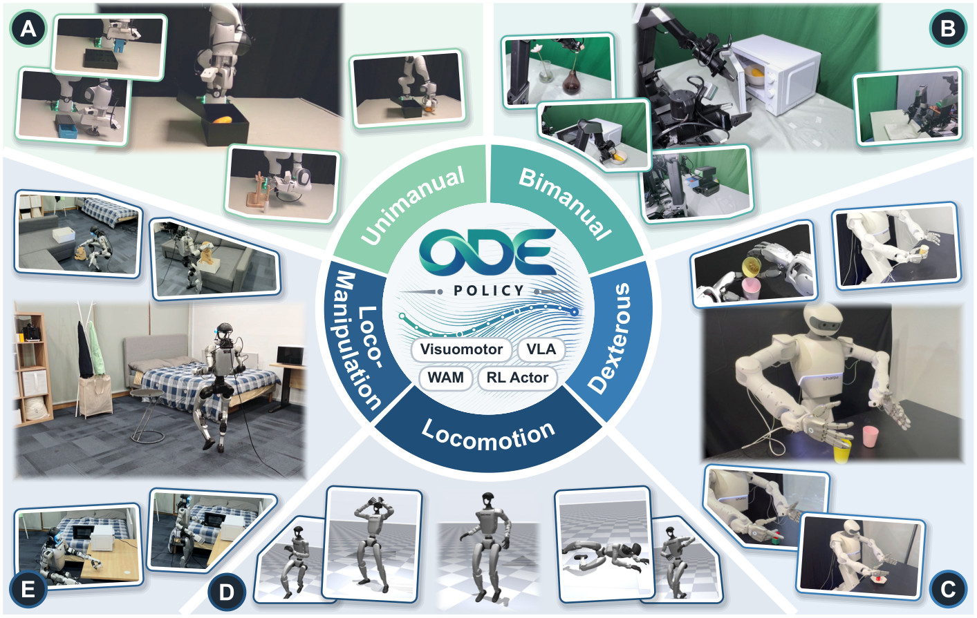
图 1:ODE 策略在不同本体和模型中的应用。同一种表述可以作为视觉运动策略、VLA 和 WAM 的动作头,以及 RL 的执行器。(A) 单臂的单手操作。(B) 双臂机器人的双手操作。(C) 五指灵巧手的灵巧操作。(D) 用 RL 训练、跟踪人类动作的仿真人形机器人运动。(E) 人形机器人的移动操作。
原图注:ODE policy across embodiments and models. The same formulation serves as a visuomotor policy, as the action head of a VLA and a WAM, and as the actor of RL. (A) Unimanual manipulation with a single arm. (B) Bimanual manipulation on a dual-arm robot. (C) Dexterous manipulation with five-fingered hands. (D) Locomotion of a simulated humanoid that tracks human motions, trained by RL. (E) Loco-manipulation with a humanoid robot.
图 1 解读
中央圆盘写着四种用法:Visuomotor(视觉运动策略)、VLA、WAM、RL Actor。周围五个扇区对应五类任务,每类配真机或仿真照片:(A) 单臂把物体放进盒子等;(B) 双臂机器人开微波炉、倒水等;(C) 人形机器人的灵巧手抓杯子、递物;(D) 仿真人形机器人模仿人类的各种动作(行走、翻滚、躺下);(E) 人形机器人在卧室环境中移动并操作。这是一张“覆盖面”展示图,具体任务和结果见第 7 节。
原文
In this work, we propose ODE policy. It learns the dynamics of the action rather than the action itself, i.e., it models the policy directly as an ODE (Fig. 2). Concretely, a neural ODE (Chen et al., 2018) learns the vector field of the action, conditioned on the observation. The action is then integrated over the physical time of the robot. Integrating over a whole demonstration accumulates drift and requires the costly adjoint method. In IL, we therefore integrate over action chunks (Chi et al., 2025; Zhao et al., 2023), a key to current direct-action policies (Pan et al., 2026; Lazzati et al., 2026), and supervise the integrated path without any derivative of the actions.
译文
在本工作中,我们提出 ODE 策略。它学习动作的动态而不是动作本身,即直接把策略建模为一个 ODE(图 2)。具体而言,一个神经 ODE(Chen et al., 2018)以观测为条件学习动作的向量场,然后在机器人的物理时间上对动作积分。在整条示范上积分会累积漂移,并且需要代价高昂的伴随(adjoint)方法。因此在 IL 中,我们在动作块上积分(Chi et al., 2025; Zhao et al., 2023)——动作块是当前直接动作策略的关键(Pan et al., 2026; Lazzati et al., 2026)——并在不使用任何动作导数的情况下监督积分得到的路径。
解释
为什么不在整条示范上积分:一条示范可能有几百步,误差会随积分步数累积(漂移),而且反向传播要穿过几百个求解步,显存放不下,只能用伴随方法(多做一次反向积分换取恒定显存),很慢。在动作块上积分:只积分 H 步(如 16 步),梯度可以直接穿过这几步,简单高效。“不使用动作导数”很关键:示范只有动作值,没有“动作的变化率”,如果用差分去估计变化率会放大噪声;作者直接比较“积分出来的路径”和“示范路径”,绕开了这个问题。
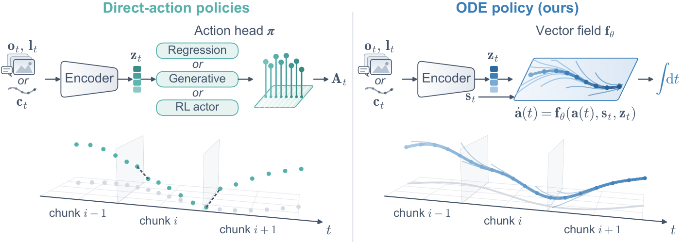
图 2:直接动作策略与 ODE 策略。二者都编码图像历史和指令(IL)或参考动作(RL)。左:直接动作策略,无论是回归头、生成式头还是 RL 的执行器,都把嵌入映射为离散控制步上的动作值。右:ODE 策略则学习动作的动态,即向量场 \mathbf{f}_\theta,并在物理时间上对其积分,使每个动作都由前一个动作推出。在 RL 中,每个动作块只含一个动作。
原图注:Direct-action policies and ODE policy. Both encode the image history and the instruction (IL) or the reference motion (RL). Left: Direct-action policies, whether a regression head, a generative head, or the actor of RL, map the embedding to action values at discrete control steps. Right: ODE policy instead learns the dynamics of the action, a vector field \mathbf{f}_\theta, and integrates it in physical time, so that each action follows from the previous one. In RL, each chunk holds a single action.
图 2 解读
上半部分是网络结构。左(直接动作策略):观测 \mathbf{o}_t、指令 \mathbf{l}_t 或条件 \mathbf{c}_t 经编码器得到嵌入 \mathbf{z}_t,再经动作头 \boldsymbol\pi(回归、生成式或 RL 执行器三选一)直接输出动作块 \mathbf{A}_t,图中画成一排独立的竖条。右(ODE 策略):同样的编码器得到 \mathbf{z}_t,但动作头换成向量场 \mathbf{f}_\theta,输入还包括本体状态 \mathbf{s}_t,公式为 \dot{\mathbf{a}}(t)=\mathbf{f}_\theta(\mathbf{a}(t),t,\mathbf{s}_t,\mathbf{z}_t),右端的 \int\mathrm{d}t 表示积分。 下半部分是动作随时间的变化。左:三个相邻动作块(i-1、i、i+1)各是一串离散的绿点,块与块之间明显错位跳变,块内也有起伏。右:一条连续平滑的蓝色曲线贯穿三个块,块边界处没有跳变,因为每块的起点就是上一块的终点。
原文
A contractive perturbation shifts the start of each training chunk and teaches the field to return, which improves robustness. In RL, we integrate over single control steps. At inference, each action is integrated from the previous one, across chunk boundaries in IL and across control steps in RL. Direct-action policies, in contrast, often jump or pause at chunk boundaries in IL and oscillate between steps in RL. Finally, a lightweight diversity head adds a sampled offset to the vector field to retain multi-modal behavior (Chi et al., 2025; Jia et al., 2026a).
译文
收缩扰动会平移每个训练动作块的起点,并教向量场把动作“拉回来”,从而提高鲁棒性。在 RL 中,我们在单个控制步上积分。推理时,每个动作都从前一个动作积分得到:在 IL 中跨越动作块边界,在 RL 中跨越控制步。相比之下,直接动作策略在 IL 中常在动作块边界处跳变或停顿,在 RL 中则在相邻步之间振荡。最后,一个轻量的多样性头给向量场加上一个采样得到的偏移,以保留多模态行为(Chi et al., 2025; Jia et al., 2026a)。
解释
三个组件:收缩扰动(训练时故意把起点挪开一点,要求轨迹回到示范上,类似“纠偏”训练,见 4.2 节);跨块积分(推理时下一块从上一块的最后一个动作接着积分,见 4.3 节);多样性头(采样一个随机偏移改变向量场方向,从而在不同模式之间选择,见 4.4 节)。“停顿”是指块边界处动作接不上时,有些实现会等待或插值。
原文
We validate ODE policy across the mainstream IL models and in RL (Fig. 1). We instantiate it as a visuomotor policy, as the action expert of the \pi_{0.5} VLA (Physical Intelligence et al., 2025), as the action head of the ImageWAM (Zhang et al., 2026) WAM, and as the actor of SuperMimic (Liao et al., 2026a) for whole-body motion tracking of a humanoid. We further deploy it on a real single-arm robot, a dual-arm robot, a robot with dexterous hands, and a humanoid, where it replaces the action head of GR00T N1.7 (Bjorck et al., 2025). The real-robot tasks include high-precision, long-horizon, deformable, multi-modal, dexterous, and loco-manipulation tasks. We compare with 14 state-of-the-art baselines, including generative and regression-based IL methods. Within each setting, all methods share the same backbone, data, and training schedule.
译文
我们在主流 IL 模型和 RL 中验证 ODE 策略(图 1)。我们把它实例化为视觉运动策略、\pi_{0.5} VLA(Physical Intelligence et al., 2025)的动作专家、ImageWAM(Zhang et al., 2026)这一 WAM 的动作头,以及用于人形机器人全身动作跟踪的 SuperMimic(Liao et al., 2026a)的执行器。我们还把它部署在真实的单臂机器人、双臂机器人、带灵巧手的机器人和人形机器人上,在后者中替换 GR00T N1.7(Bjorck et al., 2025)的动作头。真机任务包括高精度、长时程、可变形物体、多模态、灵巧操作和移动操作任务。我们与 14 个最先进的基线比较,包括生成式和基于回归的 IL 方法。在每种设定内,所有方法共享相同的主干、数据和训练日程。
解释
“共享主干、数据和训练日程”是公平比较的关键:只换动作头,其余全同。这与 StarVLA 中“只换一个模块”的思路一致。SuperMimic 是用可微分世界模型训练人形机器人动作跟踪的 RL 方法(本工作区已有译稿),这里把它的执行器网络换成 ODE 策略。
原文
Experiments show that ODE policy learns remarkably fast. After one epoch, it succeeds in 79.2% of the LIBERO episodes, against at most 43.2% for the baselines. As the action head of \pi_{0.5}, it succeeds in 96.0% against 75.5% for its flow matching expert. As that of ImageWAM, it succeeds in 82.6% against 24.6% for the original head. It matches flow matching with less than half of the demonstrations. As the actor of SuperMimic, it reaches a higher return early in training. On 14 tasks across single-arm, dual-arm, dexterous, and humanoid robots, it achieves the highest success rate on every task.
译文
实验表明,ODE 策略学得非常快。训练一个 epoch 后,它在 LIBERO 中的成功率为 79.2%,而各基线最高为 43.2%。作为 \pi_{0.5} 的动作头,它的成功率为 96.0%,而其流匹配专家为 75.5%。作为 ImageWAM 的动作头,它为 82.6%,而原动作头为 24.6%。它只用不到一半的示范就能达到流匹配的水平。作为 SuperMimic 的执行器,它在训练早期就达到更高的回报。在单臂、双臂、灵巧手和人形机器人的 14 个任务上,它在每个任务上都取得了最高成功率。
解释
注意这些对比都是在训练早期(一个 epoch 或较少训练量)进行的,衡量的是学习速度。79.2/43.2\approx1.8 倍,与摘要中“5.9 倍”不是同一个对比:摘要是与流匹配比,这里“最高 43.2%”是所有基线中最好的那个;由此推算流匹配一个 epoch 后约为 79.2/5.9\approx13.4\%,后文图 4 可以核对。
原文
It also generates actions fast and smoothly. A chunk takes 10.8 times less time than with flow matching in simulation, and 3.5 to 27 times less than with the diffusion and flow matching baselines on real robots. On real robots, its motion is smoother than the human demonstrations in most cases. Moreover, it generalizes robustly to unseen perturbations in simulation, and it transfers dexterous skills learned from public data of another lab to our real robot. It also keeps multi-modal behavior, both on a navigation task and on a real bimanual task, where it uses both arm assignments. Finally, the learned field supports data without action labels and arbitrary control rates.
译文
它还能快速、平滑地生成动作。在仿真中,生成一个动作块的时间比流匹配少 10.8 倍;在真机上,比扩散和流匹配基线少 3.5 到 27 倍。在真机上,它的运动在多数情况下比人类示范更平滑。此外,它对仿真中未见过的扰动泛化稳健,并能把从另一个实验室的公开数据中学到的灵巧技能迁移到我们的真机上。它还能保持多模态行为,无论是在导航任务上,还是在真实的双臂任务上(它会使用两种手臂分工)。最后,学到的向量场支持没有动作标签的数据和任意控制频率。
解释
为什么快:流匹配要从噪声迭代约 10 步才得到一个动作块,每步都要算一次网络;ODE 策略每个动作只需求解器的一两次函数计算(视求解器而定),而且向量场网络很小。为什么比人类示范还平滑:人手遥操作有抖动,ODE 积分有低通滤波的效果。最后一句提到的两种扩展能力(无动作标签数据、任意控制频率)在第 9 节讨论,属于展望而非主实验。
2相关工作(Related Work)
2.1机器人策略中的 ODE
原文
Action dynamics as ODEs. Representing robot motion as a dynamical system has a long history, from dynamical movement primitives (Ijspeert et al., 2013) and stable dynamical systems (Khansari-Zadeh and Billard, 2011) to neural vector fields with contraction or stability guarantees (Beik-Mohammadi et al., 2024; Sochopoulos et al., 2024). Neural dynamic policies (Bahl et al., 2020; Totsila et al., 2023) further predict the parameters of such systems from images. However, the fixed form or the stability constraint limits each system to a few motions toward an attractor, mostly on single tasks. ODE policy instead places no structural constraint on the vector field and learns one field for large-scale tasks.
译文
把动作动态建模为 ODE。把机器人运动表示为动力系统由来已久,从动态运动基元(Ijspeert et al., 2013)和稳定动力系统(Khansari-Zadeh and Billard, 2011),到具有收缩性或稳定性保证的神经向量场(Beik-Mohammadi et al., 2024; Sochopoulos et al., 2024)。神经动态策略(Bahl et al., 2020; Totsila et al., 2023)进一步从图像中预测这类系统的参数。然而,固定的形式或稳定性约束使每个系统只能表示少数几种朝向吸引子的运动,而且大多只用于单一任务。ODE 策略则对向量场不施加任何结构约束,并为大规模任务学习同一个向量场。
解释
这一类工作与本文最接近,都是“动作 = ODE 的解”。区别在于:传统方法为了保证稳定(不会发散),规定向量场必须把运动拉向某个目标点(吸引子),于是只能表达“到达某处”这类运动;ODE 策略不加约束,让一个大网络在海量多任务数据上学一个通用的向量场,稳定性改由“收缩扰动”这一训练技巧在局部提供。代价是失去了理论上的全局稳定保证。
原文
State dynamics as ODEs. A conventional paradigm in robot learning is to learn the state dynamics of the robot or its environment and then design a policy or analytical controller upon it. Learned dynamics, often in the form of neural ODEs, are used for model-based reinforcement learning (Yildiz et al., 2021) and for feedback controllers that compensate for model uncertainty (Jia et al., 2025b; Jia et al., 2025a; Jia et al., 2026b). Continuous-time networks (Hasani et al., 2022) likewise evolve the hidden state of a policy by an ODE. In these works, the ODE describes the state of the system or of the network, and the action is still produced by a separate controller or output layer. ODE policy instead learns the ODE of the action itself.
译文
把状态动态建模为 ODE。机器人学习中的一种传统范式是先学习机器人或环境的状态动态,再在其上设计策略或解析控制器。学到的动态(常以神经 ODE 的形式出现)被用于基于模型的强化学习(Yildiz et al., 2021),以及补偿模型不确定性的反馈控制器(Jia et al., 2025b; Jia et al., 2025a; Jia et al., 2026b)。连续时间网络(Hasani et al., 2022)同样用 ODE 演化策略的隐藏状态。在这些工作中,ODE 描述的是系统或网络的状态,动作仍由单独的控制器或输出层产生。ODE 策略则学习动作本身的 ODE。
解释
这是一个容易混淆的区分。状态 ODE:\dot{\mathbf x}=g(\mathbf x,\mathbf a),描述“给定动作后世界怎么变”,是世界模型。动作 ODE:\dot{\mathbf a}=f(\mathbf a,\ldots),描述“动作自身怎么变”,是策略。Jia et al. 系列是第一作者此前在神经 ODE 控制方向的工作;Hasani 等的“液态神经网络”把网络内部状态做成 ODE,但输出仍是普通的动作值。
原文
Generative processes as ODEs. Diffusion and flow matching policies (Chi et al., 2025; Black et al., 2024) integrate over a generation time without physical meaning. Streaming flow policy (Jiang et al., 2025) aligns the flow time with the execution time, but it is still trained by regressing velocities derived from the demonstrations and regenerates each chunk over a rescaled time interval. Chronos policy (Wang et al., 2026) encodes the physical times of observations and actions in a diffusion transformer, but time remains an input, and actions are still generated at a fixed rate. In contrast, ODE policy integrates over physical time itself, is trained through the integrated path without velocity labels, and continues each chunk from the previous one.
译文
把生成过程建模为 ODE。扩散和流匹配策略(Chi et al., 2025; Black et al., 2024)在一个没有物理意义的生成时间上积分。流式流策略(Streaming flow policy,Jiang et al., 2025)把流的时间与执行时间对齐,但它仍通过回归由示范导出的速度来训练,并且在一个重新缩放的时间区间上重新生成每个动作块。Chronos 策略(Wang et al., 2026)在扩散 Transformer 中编码观测和动作的物理时间,但时间仍只是一个输入,动作仍以固定频率生成。相比之下,ODE 策略在物理时间本身上积分,通过积分路径训练而无需速度标签,并让每个动作块从前一个动作块接续。
解释
最容易混淆的一点:流匹配也是“学一个向量场再积分”,为什么不一样?流匹配的积分变量 \tau\in[0,1] 是“从噪声变成动作块”的生成进度,中间状态是半噪声的动作块,机器人不能执行;ODE 策略的积分变量 t 是真实时间,积分路径上的每一点都是可执行的动作。Streaming flow policy 最接近本文,区别在于它用“示范动作的差分”作为速度标签来回归,噪声会被放大;本文只监督积分结果。
2.2动作分块
原文
Predicting a chunk of actions per observation was popularized by action chunking transformer (ACT) (Zhao et al., 2023) and diffusion policy (Chi et al., 2025), and is now standard in large foundation models (Black et al., 2024; Physical Intelligence et al., 2025; Bjorck et al., 2025). Recent analyses show that chunking is a key factor in the performance of current IL policies (Lazzati et al., 2026; Pan et al., 2026). Executing a chunk open-loop often outperforms updating the action at every observation (Park, 2026), which contrasts with the classical control experience that a higher closed-loop rate is better. However, independently predicted chunks may be inconsistent at their boundaries, which is mitigated by temporal ensembling (Zhao et al., 2023) or by conditioning each chunk on the committed actions of the previous one (Black et al., 2025).
译文
每次观测预测一个动作块的做法由动作分块 Transformer(ACT)(Zhao et al., 2023)和扩散策略(Chi et al., 2025)推广开来,如今已是大型基础模型的标准做法(Black et al., 2024; Physical Intelligence et al., 2025; Bjorck et al., 2025)。近期分析表明,分块是当前 IL 策略性能的一个关键因素(Lazzati et al., 2026; Pan et al., 2026)。以开环方式执行一个动作块,往往优于在每次观测时都更新动作(Park, 2026),这与经典控制中“闭环频率越高越好”的经验相反。然而,独立预测的动作块在边界处可能不一致,可以通过时间集成(Zhao et al., 2023)或以前一块已确定执行的动作为条件来生成下一块(Black et al., 2025)来缓解。
解释
为什么开环执行动作块反而更好:模仿学习中,示范者的动作有时间相关性(例如“先慢后快”的节奏),单步预测容易丢失这种一致性,并且对观测噪声更敏感。时间集成:每一步都预测一个动作块,同一时刻会有多个块给出预测,加权平均后执行;RTC:生成新块时把旧块中已确定要执行的动作当作约束(修补,inpainting)。这两种方法都是“事后补救”,ODE 策略则从结构上保证边界连续。
原文
ODE policy also builds on chunking for IL, but uses the chunk as the unit of integration. During training, it integrates the vector field over one chunk, so the gradient passes through a few solver steps without the adjoint method. At inference, it integrates each action from the previous one, which keeps the actions continuous across chunks and executes each action without waiting for a whole chunk. Some policies predict actions relative to the current pose (Chi et al., 2024), but still output each action of a chunk as a separate value. In ODE policy, all actions of a chunk follow from one vector field evaluated along the path.
译文
ODE 策略在 IL 中同样以分块为基础,但把动作块用作积分单位。训练时,它在一个动作块上对向量场积分,梯度只需穿过少数几个求解步,无需伴随方法。推理时,它从前一个动作积分出每个动作,从而保持跨动作块的连续性,并且无需等待整个动作块生成就能执行每个动作。有些策略预测相对于当前位姿的动作(Chi et al., 2024),但仍把动作块中的每个动作作为单独的值输出。在 ODE 策略中,一个动作块中的所有动作都由沿路径计算的同一个向量场推出。
解释
“无需等待整个动作块”:积分是逐步进行的,算出第 1 步就可以立即执行,同时继续算第 2 步,这对实时控制很有利。相对动作(如 UMI 中相对当前末端位姿的动作)与 ODE 的区别:相对动作仍是“一次输出 H 个独立偏移”,而 ODE 是“一条规则反复应用 H 次”。
2.3高效策略
原文
Efficient IL policies. Generative policies require multiple network evaluations per chunk. Consistency models (Song et al., 2023; Zhang et al., 2025), self-distillation (Li et al., 2026), and mean flows (Geng et al., 2025; Fang et al., 2025) reduce the sampling to one or a few steps, and informed source distributions shorten the transport path (Scholz and Turner, 2025; Dai et al., 2026). VITA (Gao et al., 2026), action-to-action flow matching (A2A) (Jia et al., 2026c; Zuo et al., 2026), and FLASH (Bai et al., 2026) further replace the flow source with image observations or historical actions, which improves both learning efficiency and inference speed. These methods improve the efficiency of IL within the conventional direct-action paradigm. ODE policy instead changes the paradigm to an ODE, which exploits the inherent continuity of physical motion to improve efficiency.
译文
高效的 IL 策略。生成式策略每个动作块需要多次网络计算。一致性模型(Song et al., 2023; Zhang et al., 2025)、自蒸馏(Li et al., 2026)和均值流(Geng et al., 2025; Fang et al., 2025)把采样减少到一步或少数几步,而有信息的源分布缩短了输运路径(Scholz and Turner, 2025; Dai et al., 2026)。VITA(Gao et al., 2026)、动作到动作流匹配(A2A)(Jia et al., 2026c; Zuo et al., 2026)和 FLASH(Bai et al., 2026)进一步用图像观测或历史动作替代流的源分布,同时提高了学习效率和推理速度。这些方法都是在传统直接动作范式之内提高 IL 的效率。ODE 策略则把范式换成 ODE,利用物理运动固有的连续性来提高效率。
解释
加速生成式策略的两条路:少走几步(一致性模型、均值流把 10 步压缩到 1 步);起点更近(不从纯噪声出发,而从历史动作或图像特征出发,路径更短)。A2A 和 FLASH 是本文作者团队的前作(Jia、Bai、Zuo 都是本文作者),从“历史动作出发”到“直接学动作的动态”是一条自然的思想演进。
原文
Efficient RL policies. In RL, sample efficiency is mostly improved on the side of the critic and the update, e.g., by high update-to-data ratios with ensembled or regularized critics (Chen et al., 2021b; Hiraoka et al., 2022; Bhatt et al., 2024), scaled networks (Lee et al., 2025; Kim et al., 2026), or learned world models (Hansen et al., 2024). SuperMimic (Liao et al., 2026a) learns a differentiable world model and trains the actor by backpropagating analytic gradients through short imagined rollouts. It surpasses a state-of-the-art motion tracker after 3 hours on one GPU with more than 1000 times fewer GPU hours. These methods keep the actor as a direct map from states to actions. ODE policy instead changes the actor itself, and further speeds up SuperMimic as a drop-in replacement of its actor.
译文
高效的 RL 策略。在 RL 中,样本效率大多是从评论家和更新方式的角度来提高的,例如在集成或正则化的评论家下采用高更新数据比(Chen et al., 2021b; Hiraoka et al., 2022; Bhatt et al., 2024)、扩大网络规模(Lee et al., 2025; Kim et al., 2026),或学习世界模型(Hansen et al., 2024)。SuperMimic(Liao et al., 2026a)学习一个可微分世界模型,并通过在短的想象推演中反向传播解析梯度来训练执行器。它在单张 GPU 上训练 3 小时就超过了一个最先进的动作跟踪器,所用 GPU 小时数少 1000 倍以上。这些方法都保持执行器是从状态到动作的直接映射。ODE 策略则改变执行器本身,并作为 SuperMimic 执行器的即插即用替换,进一步加快了它的训练。
解释
RL 的分工:评论家(critic)估计“这个状态/动作有多好”,执行器(actor)决定“做什么动作”。以往的提效工作大多改评论家或训练流程,本文改的是执行器的函数形式,因此与那些方法正交、可以叠加。SuperMimic 的关键是“可微分世界模型 + 解析梯度”:奖励对动作的梯度可以直接穿过世界模型传回来,不需要像 PPO 那样靠大量采样估计梯度。
3预备知识(Preliminaries)
原文
This section first formalizes the direct-action policies that ODE policy replaces, in both IL and RL, and then introduces the neural ODE on which ODE policy is built.
译文
本节首先在 IL 和 RL 两种设定下形式化 ODE 策略所要取代的直接动作策略,然后介绍 ODE 策略所基于的神经 ODE。
解释
先立“靶子”(直接动作策略的数学形式),再介绍“工具”(神经 ODE),第 4 节把二者结合。
3.1直接动作策略
原文
Let \mathbf{o}_t\in\mathcal{O} denote the visual observation in the image space \mathcal{O}, \mathbf{s}_t\in\mathbb{R}^{d_s} the proprioceptive state, and \mathbf{a}_t\in\mathbb{R}^{d_a} the action sent to the low-level controller at control step t\in\mathbb{N}, where d_s,d_a\in\mathbb{N} are the state and action dimensions. We write \mathbf{c}_t=(\mathbf{o}_t,\,\mathbf{l}_t) for the condition, with a language instruction \mathbf{l}_t\in\mathcal{T} in the space of instruction texts \mathcal{T}. The observation and the state usually include a short history. A conventional policy maps the condition and the state to the action value at each control step,
\mathbf{a}_t\sim\boldsymbol{\pi}(\cdot\mid\mathbf{c}_t,\mathbf{s}_t),(1)
where each action is predicted as a separate value. The model imposes no relation between consecutive actions. Any such relation, such as the continuity of the motion, must be learned implicitly from data. We call such policies direct-action policies, since the network outputs the action values themselves. 译文
设 \mathbf{o}_t\in\mathcal{O} 表示图像空间 \mathcal{O} 中的视觉观测,\mathbf{s}_t\in\mathbb{R}^{d_s} 表示本体感知状态,\mathbf{a}_t\in\mathbb{R}^{d_a} 表示在控制步 t\in\mathbb{N} 发送给底层控制器的动作,其中 d_s,d_a\in\mathbb{N} 分别是状态和动作的维数。记条件 \mathbf{c}_t=(\mathbf{o}_t,\,\mathbf{l}_t),其中 \mathbf{l}_t\in\mathcal{T} 是指令文本空间 \mathcal{T} 中的语言指令。观测和状态通常包含一小段历史。传统策略把条件和状态映射为每个控制步上的动作值:
\mathbf{a}_t\sim\boldsymbol{\pi}(\cdot\mid\mathbf{c}_t,\mathbf{s}_t),(1)
其中每个动作都作为单独的值预测。模型不在相邻动作之间施加任何关系。任何这样的关系,例如运动的连续性,都必须从数据中隐式学习。我们把这类策略称为直接动作策略,因为网络输出的就是动作值本身。 解释
符号对照:\mathbf o_t 是图像,\mathbf s_t 是关节角等本体状态,\mathbf l_t 是语言指令,\mathbf c_t 把图像和指令打包成“条件”。\mathbf a_t 是发给底层控制器的目标(例如目标关节角),不是机器人实际到达的位置。\sim 表示动作可以从分布中采样(生成式策略),确定性策略则直接等于网络输出。公式 (1) 的要点是:\mathbf a_t 与 \mathbf a_{t-1} 之间没有任何结构上的联系。
原文
IL policies. IL fits \boldsymbol{\pi} to a dataset \mathcal{D} of N\in\mathbb{N} demonstrated trajectories \{(\mathbf{o}_t,\mathbf{s}_t,\mathbf{l}_t,\mathbf{a}_t)\}. Most IL policies follow action chunking (Zhao et al., 2023; Chi et al., 2025) and predict a chunk of H\in\mathbb{N} future actions at once,
\mathbf{A}_t=[\mathbf{a}_{t},\dots,\mathbf{a}_{t+H-1}]\sim\boldsymbol{\pi}(\cdot\mid\mathbf{c}_t,\mathbf{s}_t),(2)
with \mathbf{A}_t\in\mathbb{R}^{H\times d_a}, which is executed before the next observation is processed. Each action \mathbf{a}_{t+k} with k\in\{0,\dots,H-1\} is still a separate value, within and across chunks, and H=1 recovers Eq. (1). Explicit regression maps (\mathbf{c}_t,\mathbf{s}_t) directly to \mathbf{A}_t under an \ell_1 or \ell_2 loss (Pomerleau, 1989; Zhao et al., 2023), which is simple but averages multi-modal demonstrations. Generative policies instead sample \mathbf{A}_t from a learned distribution. Diffusion policies (Chi et al., 2025; Ho et al., 2020) iteratively denoise a chunk drawn from Gaussian noise, and flow matching policies (Lipman et al., 2023; Liu et al., 2023b; Black et al., 2024; Jia et al., 2026c) integrate a deterministic vector field that transports a source sample to \mathbf{A}_t over a time \tau\in[0,1]. 译文
IL 策略。IL 把 \boldsymbol{\pi} 拟合到一个包含 N\in\mathbb{N} 条示范轨迹 \{(\mathbf{o}_t,\mathbf{s}_t,\mathbf{l}_t,\mathbf{a}_t)\} 的数据集 \mathcal{D} 上。大多数 IL 策略采用动作分块(Zhao et al., 2023; Chi et al., 2025),一次预测 H\in\mathbb{N} 个未来动作组成的动作块:
\mathbf{A}_t=[\mathbf{a}_{t},\dots,\mathbf{a}_{t+H-1}]\sim\boldsymbol{\pi}(\cdot\mid\mathbf{c}_t,\mathbf{s}_t),(2)
其中 \mathbf{A}_t\in\mathbb{R}^{H\times d_a},它在处理下一次观测之前执行完毕。对 k\in\{0,\dots,H-1\},每个动作 \mathbf{a}_{t+k} 无论在块内还是跨块,仍然是一个单独的值;取 H=1 即退化为公式 (1)。显式回归在 \ell_1 或 \ell_2 损失下把 (\mathbf{c}_t,\mathbf{s}_t) 直接映射为 \mathbf{A}_t(Pomerleau, 1989; Zhao et al., 2023),这种做法简单,但会把多模态示范平均掉。生成式策略则从学到的分布中采样 \mathbf{A}_t。扩散策略(Chi et al., 2025; Ho et al., 2020)对从高斯噪声中采样的动作块进行迭代去噪;流匹配策略(Lipman et al., 2023; Liu et al., 2023b; Black et al., 2024; Jia et al., 2026c)则在时间 \tau\in[0,1] 上对一个确定性向量场积分,把源样本输运到 \mathbf{A}_t。 解释
三种直接动作头的对比:回归(ACT、OpenVLA-OFT):一次前向输出,快,但遇到“向左或向右都对”的数据会输出“向前”撞上障碍;扩散:迭代去噪,能表达多模态,但慢;流匹配(\pi_0):学一个从噪声到动作块的“传送带”,比扩散步数少,但仍需约 10 步。Pomerleau (1989) 的 ALVINN 是最早的端到端行为克隆自动驾驶系统。
原文
Notably, although diffusion and flow matching solve a differential equation at inference, \tau is a generation time without physical meaning. The intermediate sample is not a state the robot can occupy, and each chunk is generated anew, independently of where the previous chunk ended.
译文
值得注意的是,尽管扩散和流匹配在推理时也在求解微分方程,但 \tau 是一个没有物理意义的生成时间。中间样本并不是机器人可以处于的状态,而且每个动作块都重新生成,与前一个动作块在哪里结束无关。
解释
这一段专门澄清“流匹配也是 ODE”可能带来的混淆。可以用一个比喻:流匹配像在暗房里冲洗一整张照片(\tau 是显影进度,中间是模糊的半成品);ODE 策略像用笔沿着时间一笔画下去(t 是真实时间,每一刻笔尖都在纸上某处)。
原文
RL policies. RL instead trains \boldsymbol{\pi} through interaction to maximize the expected discounted return. Without images, \mathbf{s}_t holds the state history, and for motion tracking the condition \mathbf{c}_t holds the reference motion. The actor typically outputs a single action at each control step as in Eq. (1). Model-based methods such as SuperMimic (Liao et al., 2026a) update the actor by backpropagating the return of rollouts imagined in a differentiable world model.
译文
RL 策略。RL 则通过交互训练 \boldsymbol{\pi},以最大化期望折扣回报。没有图像时,\mathbf{s}_t 包含状态历史;对于动作跟踪,条件 \mathbf{c}_t 包含参考动作。执行器通常按公式 (1) 在每个控制步输出单个动作。SuperMimic(Liao et al., 2026a)等基于模型的方法,通过反向传播在可微分世界模型中想象推演的回报来更新执行器。
解释
期望折扣回报:\mathbb E[\sum_t\gamma^t r_t],\gamma<1 让近期奖励更重要。动作跟踪任务中,条件是一段人类动作捕捉数据(参考动作),机器人要尽量模仿它。RL 中不做动作分块(H=1),所以 ODE 策略在 RL 中只积分一步(第 4.5 节)。
3.2神经 ODE
原文
A neural ODE (Chen et al., 2018; Jia et al., 2025b) parameterizes the time derivative of a continuous state \mathbf{x}(t)\in\mathbb{R}^{n}, n\in\mathbb{N}, at time t\in\mathbb{R} with a neural network \mathbf{g}_\phi:\mathbb{R}^{n}\times\mathbb{R}\to\mathbb{R}^{n} with parameters \phi, and obtains its trajectory from t_0 to t_1 (t_0,t_1\in\mathbb{R}, t_0<t_1) by integration,
\dot{\mathbf{x}}(t)=\mathbf{g}_\phi\big(\mathbf{x}(t),t\big),\qquad \mathbf{x}(t_1)=\mathbf{x}(t_0)+\int_{t_0}^{t_1}\mathbf{g}_\phi\big(\mathbf{x}(t),t\big)\,\mathrm{d}t ,(3)
where the integral is evaluated by a numerical solver (e.g., the Euler method or Runge–Kutta methods such as RK2 and RK4) and the network is trained by back-propagating a loss on the integrated states. 译文
神经 ODE(Chen et al., 2018; Jia et al., 2025b)用一个参数为 \phi 的神经网络 \mathbf{g}_\phi:\mathbb{R}^{n}\times\mathbb{R}\to\mathbb{R}^{n} 参数化连续状态 \mathbf{x}(t)\in\mathbb{R}^{n}(n\in\mathbb{N})在时间 t\in\mathbb{R} 的时间导数,并通过积分得到从 t_0 到 t_1(t_0,t_1\in\mathbb{R},t_0<t_1)的轨迹:
\dot{\mathbf{x}}(t)=\mathbf{g}_\phi\big(\mathbf{x}(t),t\big),\qquad \mathbf{x}(t_1)=\mathbf{x}(t_0)+\int_{t_0}^{t_1}\mathbf{g}_\phi\big(\mathbf{x}(t),t\big)\,\mathrm{d}t ,(3)
其中积分由数值求解器计算(例如欧拉法,或 RK2、RK4 等龙格—库塔法),网络通过对积分得到的状态上的损失进行反向传播来训练。 解释
公式 (3) 的两部分:左式说“\mathbf x 的变化率由网络 \mathbf g_\phi 决定”;右式说“终点 = 起点 + 变化率的累积”。数值求解器:欧拉法最简单,\mathbf x(t+\Delta)\approx\mathbf x(t)+\Delta\cdot\mathbf g(\mathbf x(t),t),每步算一次网络;RK2 每步算两次(先试走半步再修正),RK4 每步算四次,精度依次提高。ODE 策略推理快不快,很大程度取决于选哪种求解器(第 8 节有消融)。
原文
The gradient is obtained either directly through the solver steps or by the adjoint method (Chen et al., 2018), which integrates an augmented ODE backward in time with constant memory at the cost of additional integration. The network only specifies the local rate of change, while the continuity and smoothness of the trajectory come from integration. Earlier robot policies built on dynamical systems, such as movement primitives (Ijspeert et al., 2013), stable dynamical systems (Khansari-Zadeh and Billard, 2011), and neural dynamic policies (Bahl et al., 2020), fix the form of the vector field in advance and learn only its parameters. In this work, we instead let the network itself be the vector field of the action, integrated over the physical time of the robot.
译文
梯度要么直接穿过求解步得到,要么通过伴随方法(Chen et al., 2018)得到;后者以额外的积分为代价,沿时间反向积分一个增广 ODE,所需内存恒定。网络只规定局部的变化率,而轨迹的连续性和平滑性来自积分。早期基于动力系统的机器人策略,如运动基元(Ijspeert et al., 2013)、稳定动力系统(Khansari-Zadeh and Billard, 2011)和神经动态策略(Bahl et al., 2020),都事先固定向量场的形式,只学习其参数。在本工作中,我们则让网络本身成为动作的向量场,并在机器人的物理时间上积分。
解释
两种求梯度方式:直接穿过求解步,就像普通的循环神经网络反向传播,显存随步数线性增长,但实现简单、梯度精确;伴随方法反向再积分一次求梯度,显存恒定,但计算量翻倍且数值误差更大。ODE 策略只积分 H 步(例如 16 步),所以直接反向传播完全可行。“连续性来自积分”是全文反复强调的观点:网络输出哪怕有些噪声,积分后也会被平滑。
4方法(Method)
原文
In this section, we propose ODE policy, which models how the action evolves over the physical time of the robot as an ODE (Fig. 2). We present it mainly for IL. We first formulate the policy as a vector field of the action (Section 4.1), then describe how it is trained from demonstrations (Section 4.2) and executed at inference (Section 4.3). Section 4.4 adds an optional diversity head for multi-modal behavior. Finally, Section 4.5 describes how the same field serves as the actor in RL.
译文
本节提出 ODE 策略,它把动作如何随机器人的物理时间演化建模为一个 ODE(图 2)。我们主要针对 IL 进行介绍。首先把策略表述为动作的向量场(第 4.1 节),然后介绍如何从示范中训练它(第 4.2 节)以及推理时如何执行(第 4.3 节)。第 4.4 节加入一个用于多模态行为的可选多样性头。最后,第 4.5 节介绍同一个向量场如何作为 RL 中的执行器。
解释
方法的五个部分:表述(公式 4、5)、训练(公式 6–8、算法 1)、推理(算法 2)、多样性头(公式 9、10)、RL(公式 11)。
4.1向量场表述
原文
Vector field. We encode the image history and the instruction into an embedding \mathbf{z}_t\in\mathbb{R}^{d_z}, d_z\in\mathbb{N}, and parameterize the velocity of the action with a neural network (Chen et al., 2018),
\dot{\mathbf{a}}(t)=\mathbf{f}_\theta\big(\mathbf{a}(t),\mathbf{s}_t,\mathbf{z}_t\big),(4)
where \mathbf{f}_\theta:\mathbb{R}^{d_a}\times\mathbb{R}^{d_s}\times\mathbb{R}^{d_z}\to\mathbb{R}^{d_a}, t\in\mathbb{R}_{\ge0} is the physical time of the robot in units of control steps, \mathbf{a}(t)\in\mathbb{R}^{d_a} is an action the robot is commanded to reach and \dot{\mathbf{a}} is its velocity. The proprioception \mathbf{s}_t enters the field directly rather than being encoded into \mathbf{z}_t together with \mathbf{c}_t as in conventional policies (ablated in Section 8). 译文
向量场。我们把图像历史和指令编码为嵌入 \mathbf{z}_t\in\mathbb{R}^{d_z}(d_z\in\mathbb{N}),并用一个神经网络参数化动作的速度(Chen et al., 2018):
\dot{\mathbf{a}}(t)=\mathbf{f}_\theta\big(\mathbf{a}(t),\mathbf{s}_t,\mathbf{z}_t\big),(4)
其中 \mathbf{f}_\theta:\mathbb{R}^{d_a}\times\mathbb{R}^{d_s}\times\mathbb{R}^{d_z}\to\mathbb{R}^{d_a},t\in\mathbb{R}_{\ge0} 是以控制步为单位的机器人物理时间,\mathbf{a}(t)\in\mathbb{R}^{d_a} 是机器人被指令到达的动作,\dot{\mathbf{a}} 是其速度。本体感知 \mathbf{s}_t 直接进入向量场,而不是像传统策略那样与 \mathbf{c}_t 一起编码进 \mathbf{z}_t(第 8 节对此做了消融)。 解释
公式 (4) 的三个输入:当前动作 \mathbf a(t)(“我现在在哪”),本体状态 \mathbf s_t(“机器人实际在哪”),视觉语言嵌入 \mathbf z_t(“要干什么、环境如何”);输出是动作的变化速度。与公式 (3) 相比,这里没有显式的 t 输入,即向量场是时不变(自治)的:同样的动作和条件,无论在动作块的第几步,变化方向都一样。时间单位是“控制步”,即 t=1 对应一个控制周期(例如 1/10 秒)。 举例:机械臂要伸手抓杯子,\mathbf z_t 编码了“杯子在前方 20 厘米”,\mathbf a(t) 是当前的目标位置;向量场在离杯子远时给出较大的前进速度,接近时速度变小,于是积分出一条先快后慢、平滑接近的轨迹。
原文
Chunked integration. At a decision step t, the policy computes \mathbf{z}_t once and holds \mathbf{z}_t and \mathbf{s}_t fixed over the chunk. Starting from the last action \hat{\mathbf{a}}_{t-1}\in\mathbb{R}^{d_a}, it integrates Eq. (4) with a numerical solver,
\hat{\mathbf{a}}_{t+k}=\hat{\mathbf{a}}_{t+k-1} +\int_{t+k-1}^{t+k}\mathbf{f}_\theta\big(\mathbf{a}(t'),\mathbf{s}_t,\mathbf{z}_t\big)\,\mathrm{d}t', \qquad k=0,\dots,H-1,(5)
where t'\in\mathbb{R} is the integration variable, and we obtain the chunk \hat{\mathbf{A}}_t=[\hat{\mathbf{a}}_{t},\dots,\hat{\mathbf{a}}_{t+H-1}]\in\mathbb{R}^{H\times d_a} at the same steps as \mathbf{A}_t in Eq. (2). In contrast to Eqs. (1) and (2), each action is obtained from the previous one by integrating its rate of change, so consecutive actions are related by construction. 译文
分块积分。在决策步 t,策略计算一次 \mathbf{z}_t,并在整个动作块内保持 \mathbf{z}_t 和 \mathbf{s}_t 不变。从上一个动作 \hat{\mathbf{a}}_{t-1}\in\mathbb{R}^{d_a} 出发,它用数值求解器对公式 (4) 积分:
\hat{\mathbf{a}}_{t+k}=\hat{\mathbf{a}}_{t+k-1} +\int_{t+k-1}^{t+k}\mathbf{f}_\theta\big(\mathbf{a}(t'),\mathbf{s}_t,\mathbf{z}_t\big)\,\mathrm{d}t', \qquad k=0,\dots,H-1,(5)
其中 t'\in\mathbb{R} 是积分变量,由此得到与公式 (2) 中 \mathbf{A}_t 处于相同时间步的动作块 \hat{\mathbf{A}}_t=[\hat{\mathbf{a}}_{t},\dots,\hat{\mathbf{a}}_{t+H-1}]\in\mathbb{R}^{H\times d_a}。与公式 (1) 和 (2) 不同,每个动作都通过对其变化率积分从前一个动作得到,因此相邻动作在结构上就是相关的。 解释
公式 (5) 用欧拉法写出来就是 \hat{\mathbf a}_{t+k}=\hat{\mathbf a}_{t+k-1}+\mathbf f_\theta(\hat{\mathbf a}_{t+k-1},\mathbf s_t,\mathbf z_t),即“下一个动作 = 当前动作 + 网络给出的增量”,重复 H 次。这看起来像一个循环网络:大的视觉编码器每块只算一次,小的向量场网络每步算一次,所以总计算量很小。帽子符号 \hat{\cdot} 表示模型预测值,不带帽子的是示范值。
原文
Notably, the field takes the current action \mathbf{a}(t) as input, so the change at each step depends on where the action has arrived. A conventional policy instead outputs the actions or increments of a chunk as H separate values, whose relation must be learned from data. Holding the condition fixed matches action chunking (Zhao et al., 2023; Chi et al., 2025), where the observation is processed once per chunk (Lazzati et al., 2026).
译文
值得注意的是,向量场以当前动作 \mathbf{a}(t) 为输入,因此每一步的变化取决于动作已经到达了哪里。传统策略则把一个动作块的动作或增量作为 H 个单独的值输出,它们之间的关系必须从数据中学习。保持条件不变与动作分块的做法一致(Zhao et al., 2023; Chi et al., 2025),即每个动作块只处理一次观测(Lazzati et al., 2026)。
解释
“以当前动作为输入”是与“预测增量”的本质区别。如果一个策略一次输出 H 个增量 [\Delta_1,\ldots,\Delta_H],第 5 个增量并不知道前 4 个累加后到了哪里;ODE 策略每算一步都“看一眼”当前位置再决定下一步,相当于块内也有一个内部闭环(尽管条件 \mathbf z_t 不变)。这也是第 4.2 节“收缩扰动”能起作用的前提。
原文
Note that the integrated state is the desired action, i.e., the target sent to the low-level controller, rather than the measured state of the robot. Since the low-level controller, e.g., a proportional-derivative (PD) or operational space controller (Khatib, 1987), tracks its target imperfectly, the robot state always lags behind the target (Zhao et al., 2026). For a delta controller (Zhu et al., 2020), the desired action is the current pose plus the scaled command, from which the command is recovered exactly at execution. When only the measured state is available, e.g., data collected by UMI (Chi et al., 2024) or from human videos (Kareer et al., 2026), we discuss how the velocity of the field naturally compensates for the lag in Section 9.
译文
注意,积分的状态是期望动作,即发送给底层控制器的目标,而不是机器人的实测状态。由于底层控制器(例如比例—微分(PD)控制器或操作空间控制器(Khatib, 1987))对目标的跟踪并不完美,机器人状态总是滞后于目标(Zhao et al., 2026)。对于增量控制器(Zhu et al., 2020),期望动作是当前位姿加上缩放后的指令,执行时可以从中精确恢复指令。当只有实测状态可用时,例如用 UMI 采集的数据(Chi et al., 2024)或来自人类视频的数据(Kareer et al., 2026),我们在第 9 节讨论向量场的速度如何自然地补偿这种滞后。
解释
目标与实际的区别:控制器收到“去 (0.5, 0.2, 0.3)”后,机械臂要花时间才能到,其间实际位置一直落后于目标。ODE 积分的是“目标序列”,不是“实际位置序列”,所以积分起点用的是上一个目标而非实测位姿,二者不会互相干扰。增量控制器(如 robosuite 中的 OSC delta 模式)的指令是“相对当前位置移动多少”,作者把它换算成“当前位置 + 增量 = 期望目标”来积分,执行时再减回去得到增量。
4.2训练
原文
Path loss. Given a demonstration segment, we start from the demonstrated action \mathbf{a}_{t-1}, integrate Eq. (5) for H steps, and match the integrated path,
\mathcal{L}_{\text{path}}=\frac{1}{H}\sum_{k=0}^{H-1} \big\|\hat{\mathbf{a}}_{t+k}-\mathbf{a}_{t+k}\big\|_2^2 .(6)
Since the chunk is usually short, the gradient is back-propagated directly through the solver steps without the adjoint method (Chen et al., 2018). The field is supervised only through the integrated path and never regressed against velocity labels as in Jiang et al. (2025), which may amplify the jitter of noisy demonstrations. 译文
路径损失。给定一个示范片段,我们从示范动作 \mathbf{a}_{t-1} 出发,对公式 (5) 积分 H 步,并匹配积分得到的路径:
\mathcal{L}_{\text{path}}=\frac{1}{H}\sum_{k=0}^{H-1} \big\|\hat{\mathbf{a}}_{t+k}-\mathbf{a}_{t+k}\big\|_2^2 .(6)
由于动作块通常很短,梯度直接穿过求解步反向传播,无需伴随方法(Chen et al., 2018)。向量场只通过积分路径受到监督,从不像 Jiang et al. (2025) 那样对速度标签进行回归,后者可能放大带噪示范中的抖动。 解释
公式 (6) 是“积分轨迹”与“示范轨迹”逐点距离平方的平均,形式上和普通回归的均方误差一样,区别在于预测值 \hat{\mathbf a}_{t+k} 是积分出来的,第 k 个点的误差会通过链式法则影响前面所有步的向量场。 为什么不用速度标签:若示范为 [1.00, 1.02, 0.99, 1.03](含噪声),差分得到的速度是 [0.02,-0.03,0.04],正负来回跳,噪声被放大了;而位置本身的误差只有 \pm0.02。直接拟合位置路径,相当于让网络自己找一条平滑的速度来解释带噪的位置,起到去噪作用。这也解释了为何 ODE 策略的运动“比人类示范更平滑”。
原文
Contractive perturbation. The path loss supervises the vector field only along the demonstrated trajectories. At execution, however, the policy integrates from its own previous output, so any error carries over to the next step and the next chunk, and the state gradually leaves the demonstrations. To improve robustness, we perturb the start point of a segment during training and require the integrated path to return to the demonstration,
\mathcal{L}_{\text{path}}^{\boldsymbol{\delta}}=\frac{1}{H}\sum_{k=0}^{H-1} \big\|\hat{\mathbf{a}}_{t+k}(\mathbf{a}_{t-1}+\boldsymbol{\delta}) -(\mathbf{a}_{t+k}+\rho^{k+1}\boldsymbol{\delta})\big\|_2^2, \qquad \boldsymbol{\delta}\sim\mathcal{N}\big(\mathbf{0},\mathrm{diag}(\boldsymbol{\sigma}_\delta^2)\big),(7)
where \hat{\mathbf{a}}_{t+k}(\cdot) denotes the path of Eq. (5) integrated from the given start point, \boldsymbol{\delta}\in\mathbb{R}^{d_a} is the perturbation with scale \boldsymbol{\sigma}_\delta\in\mathbb{R}^{d_a}_{>0}, and \rho\in(0,1) is a decay rate. Each segment is perturbed with probability p\in[0,1], and \boldsymbol{\delta}=\mathbf{0} otherwise, which recovers Eq. (6). 译文
收缩扰动。路径损失只沿示范轨迹监督向量场。然而在执行时,策略从自己上一次的输出开始积分,因此任何误差都会传递到下一步和下一个动作块,状态会逐渐偏离示范。为了提高鲁棒性,我们在训练时扰动片段的起点,并要求积分路径回到示范上:
\mathcal{L}_{\text{path}}^{\boldsymbol{\delta}}=\frac{1}{H}\sum_{k=0}^{H-1} \big\|\hat{\mathbf{a}}_{t+k}(\mathbf{a}_{t-1}+\boldsymbol{\delta}) -(\mathbf{a}_{t+k}+\rho^{k+1}\boldsymbol{\delta})\big\|_2^2, \qquad \boldsymbol{\delta}\sim\mathcal{N}\big(\mathbf{0},\mathrm{diag}(\boldsymbol{\sigma}_\delta^2)\big),(7)
其中 \hat{\mathbf{a}}_{t+k}(\cdot) 表示从给定起点按公式 (5) 积分得到的路径,\boldsymbol{\delta}\in\mathbb{R}^{d_a} 是尺度为 \boldsymbol{\sigma}_\delta\in\mathbb{R}^{d_a}_{>0} 的扰动,\rho\in(0,1) 是衰减率。每个片段以概率 p\in[0,1] 被扰动,否则 \boldsymbol{\delta}=\mathbf{0},此时退化为公式 (6)。 解释
问题:这是模仿学习经典的“复合误差”(compounding error):一旦偏离示范,模型就进入没见过的状态,越错越远。ODE 策略因为“从自己的输出接着积分”,对此尤其敏感。 做法:训练时把起点随机挪开 \boldsymbol\delta,目标也不是让第一步立刻回到示范(那会是一个跳变),而是让偏差按 \rho^{k+1} 的比例逐步缩小。算一个例子:取 \rho=0.8、\delta=1 厘米,则目标偏差依次为 0.8、0.64、0.51、0.41……厘米,16 步后约 0.03 厘米,平滑地回到示范轨迹。\mathrm{diag}(\boldsymbol\sigma_\delta^2) 表示各维独立的高斯噪声,每维尺度可以不同(例如位置和夹爪用不同尺度)。
原文
Since the target deviation \rho^{k+1}\boldsymbol{\delta} shrinks geometrically, the field learns to pull nearby states back to the demonstration at a rate set by \rho, i.e., a local contraction (Beik-Mohammadi et al., 2024) around the demonstrations. We therefore call it contractive perturbation. It relies on the field taking the action as input. Standard direct-action policies do not take the commanded action as input, so such a perturbation has no counterpart for them. The perturbation requires neither additional data nor additional computation at inference (ablated in Fig. 17(A)).
译文
由于目标偏差 \rho^{k+1}\boldsymbol{\delta} 按几何级数缩小,向量场学会以由 \rho 决定的速率把附近的状态拉回示范,即在示范周围形成局部收缩(Beik-Mohammadi et al., 2024)。因此我们称之为收缩扰动。它依赖于向量场以动作为输入。标准的直接动作策略不以指令动作为输入,因此没有与之对应的扰动方式。这一扰动既不需要额外数据,也不需要额外的推理计算(消融见图 17(A))。
解释
收缩(contraction)是动力系统术语:附近的轨迹随时间相互靠拢。这里只在示范附近“局部”成立,不是全局保证。与 DART、数据增强等方法相比,收缩扰动的好处是不需要专家额外标注“偏离后该怎么纠正”,纠正目标由公式自动生成。“直接动作策略没有对应做法”是因为它们的输入里没有“当前指令动作”,扰动无处施加;虽然可以扰动本体状态 \mathbf s_t,但效果不同。
原文
The losses above are defined on a single demonstration segment \xi_t=(\mathbf{c}_t,\mathbf{s}_t,\mathbf{a}_{t-1:t+H-1}). The total objective averages them over the segments in \mathcal{D} and the perturbations,
\mathcal{L}(\theta,\psi)=\mathbb{E}_{\xi_t\sim\mathcal{D},\,\boldsymbol{\delta}} \big[\mathcal{L}_{\text{path}}^{\boldsymbol{\delta}}(\xi_t)+\underbrace{\mathcal{L}_{\text{div}}(\xi_t)}_{\text{\textit{optional}}}\big],(8)
which is minimized over mini-batches of segments, where the optional diversity loss \mathcal{L}_{\text{div}} is introduced in Section 4.4. Algorithm 1 contrasts this training with that of a direct-action policy. 译文
上述损失定义在单个示范片段 \xi_t=(\mathbf{c}_t,\mathbf{s}_t,\mathbf{a}_{t-1:t+H-1}) 上。总目标对 \mathcal{D} 中的片段和扰动取平均:
\mathcal{L}(\theta,\psi)=\mathbb{E}_{\xi_t\sim\mathcal{D},\,\boldsymbol{\delta}} \big[\mathcal{L}_{\text{path}}^{\boldsymbol{\delta}}(\xi_t)+\underbrace{\mathcal{L}_{\text{div}}(\xi_t)}_{\text{\textit{可选}}}\big],(8)
它在片段的小批量上被最小化,其中可选的多样性损失 \mathcal{L}_{\text{div}} 在第 4.4 节介绍。算法 1 对比了这种训练方式与直接动作策略的训练方式。 解释
一个片段需要 H+1 个动作:\mathbf a_{t-1} 作积分起点,\mathbf a_t\ldots\mathbf a_{t+H-1} 作监督目标。\psi 是第 4.4 节多样性头的参数。算法 1 的对比显示 ODE 策略的训练循环只多了两行:加扰动、积分。
算法 1:IL 训练伪代码(原文 Algorithm 1: IL training pseudocode)
直接动作策略
1:for \mathcal{D} 中的每个片段 (\mathbf{c}_t,\mathbf{s}_t,\mathbf{A}_t) do
2: 更新 \theta 以拟合 \mathbf{A}_t ▷ 回归或生成
3:end for
ODE 策略
1:for \mathcal{D} 中的每个片段 (\mathbf{c}_t,\mathbf{s}_t,\mathbf{a}_{t-1:t+H-1}) do
2: \hat{\mathbf{a}}_{t-1}\gets\mathbf{a}_{t-1}+\boldsymbol{\delta} ▷ 收缩扰动
3: 从 \hat{\mathbf{a}}_{t-1} 出发对 \mathbf{f}_\theta 积分 H 步
4: 穿过求解器用 \mathcal{L}_{\text{path}}^{\boldsymbol{\delta}} 更新 \theta
5:end for
算法 1 解读
左右两栏是原文的英文伪代码的直译(原文左栏注释为 “regressed or generated”,右栏注释为 “contractive perturbation”)。关键差别:直接动作策略的监督目标是整个动作块 \mathbf A_t;ODE 策略还需要块前一步的动作 \mathbf a_{t-1} 作为起点,并且梯度要“穿过求解器”。实现上,第 3 行就是一个长度为 H 的循环,第 4 行由自动微分框架自动完成。
4.3推理
原文
At inference, each action within a chunk is obtained from the previous one by a single integration step (Algorithm 2). Across chunks, we use seamless chunking, i.e., each chunk is integrated with Eq. (5) from the last action of the previous one, \hat{\mathbf{a}}_{t-1}, rather than from the measured state (ablated in Fig. 17(B, C)). This inference gives three benefits over direct-action policies.
译文
推理时,动作块内的每个动作都通过一次积分步从前一个动作得到(算法 2)。在动作块之间,我们使用无缝分块,即每个动作块都从前一块的最后一个动作 \hat{\mathbf{a}}_{t-1} 出发按公式 (5) 积分,而不是从实测状态出发(消融见图 17(B, C))。与直接动作策略相比,这种推理方式有三个好处。
解释
为什么不从实测状态出发:上文说过,实测状态总是滞后于指令目标;如果每块都从实测状态重新开始,新块的起点就会比上一块的终点“往回退”一段,造成跳变或停顿。从上一个指令出发,指令序列就是一条连续的曲线。代价是若控制器跟踪误差持续累积(例如被外力卡住),指令可能与实际状态越离越远,但向量场的输入里还有本体状态 \mathbf s_t,可以感知这种偏差。
原文
(i) Smooth execution. Unlike independently generated chunks (Zhao et al., 2023; Black et al., 2025), successive chunks join without jumps, so the executed trajectory is a single integral curve whose condition is refreshed every H steps. (ii) Streaming execution. Each action is sent to the controller as soon as it is integrated, whereas direct-action policies must generate the whole chunk before executing its first action. (iii) Free integration step. Since the field is defined in continuous time, the integration step can be chosen at deployment, e.g., to match a higher control rate, whereas direct-action policies output actions at the fixed step of their training data (Fig. 19(C)).
译文
(i) 平滑执行。与独立生成的动作块(Zhao et al., 2023; Black et al., 2025)不同,相邻动作块之间没有跳变地衔接,因此执行出的轨迹是一条积分曲线,其条件每 H 步刷新一次。(ii) 流式执行。每个动作一经积分就立即发送给控制器,而直接动作策略必须生成整个动作块后才能执行其第一个动作。(iii) 自由选择积分步长。由于向量场定义在连续时间上,积分步长可以在部署时选择,例如匹配更高的控制频率,而直接动作策略只能以训练数据的固定步长输出动作(图 19(C))。
解释
三个好处的直观理解:(i) 轨迹整体是一条曲线,只是每隔 H 步“换一次方向盘指令”(条件 \mathbf z_t 刷新),但位置不会跳;(ii) 像流媒体边下边播,第一个动作几乎没有等待时间;(iii) 训练时步长为 1 个控制步(如 10 Hz),部署时可以用步长 0.5 积分,得到 20 Hz 的动作,而直接动作策略要做到这一点只能插值。严格说 (iii) 隐含一个假设:向量场在训练步长之间的行为也是合理的,第 9 节有初步验证。
算法 2:IL 推理伪代码(原文 Algorithm 2: IL inference pseudocode)
直接动作策略
1:for 每个决策步 t=0,H,2H,\dots do
2: \hat{\mathbf{A}}_t\sim\boldsymbol{\pi}(\cdot\mid\mathbf{c}_t,\mathbf{s}_t) ▷ 一个新动作块
3: 执行 \hat{\mathbf{A}}_t ▷ 整块生成完之后
4:end for
ODE 策略
1:for 每个决策步 t=0,H,2H,\dots do
2:for k=0,\dots,H-1 do
3: \hat{\mathbf{a}}\gets\text{Step}(\mathbf{f}_\theta,\hat{\mathbf{a}},\mathbf{s}_t,\mathbf{z}_t),发送 \hat{\mathbf{a}} ▷ 流式
4:end for
5:end for \triangleright 下一块从 \hat{\mathbf{a}} 开始
算法 2 解读
原文注释依次为 “a new chunk”“once it is complete”“streaming”“next chunk starts from \hat{\mathbf a}”。Step 表示求解器的一步(欧拉一次网络计算,RK4 四次)。注意算法中没有画出每个决策步开始时编码 \mathbf z_t 的那一步;\hat{\mathbf a} 在外层循环之间不重置,这就是“无缝分块”。
4.4用于多模态的多样性头
原文
Multi-modal behavior means that several distinct actions are valid in the same situation, e.g., passing an obstacle on the left or on the right (Chi et al., 2025; Jia et al., 2026a; Ma et al., 2026). A deterministic field \mathbf{f}_\theta fits the mean velocity of the demonstrations and thus averages such modes, e.g., heading straight into the obstacle (Fig. 3(A)).
译文
多模态行为指在同一情境下有几种不同的动作都是有效的,例如从左侧或右侧绕过障碍物(Chi et al., 2025; Jia et al., 2026a; Ma et al., 2026)。确定性向量场 \mathbf{f}_\theta 拟合的是示范的平均速度,因此会把这些模式平均掉,例如径直撞向障碍物(图 3(A))。
解释
这是回归类方法的经典问题:均方误差的最优解是条件均值。一半示范向左、一半向右,平均就是正前方。ODE 策略的路径损失本质上也是回归,所以面临同样的问题。
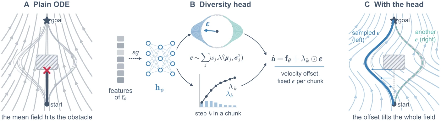
图 3:用于多模态的多样性头。示范(灰色)从左侧或右侧绕过障碍物。(A) 普通向量场把它们平均,撞上障碍物。(B) 多样性头采样一个方向 \boldsymbol{\epsilon}(每条路线一个模式)和每一步的速率 \boldsymbol{\lambda}_k,并把 \boldsymbol{\lambda}_k\odot\boldsymbol{\epsilon} 加到速度上。(C) 偏移使整个向量场倾斜,因此每个样本走一条路线。
原图注:Diversity head for multi-modality. Demonstrations (gray) pass an obstacle on the left or the right. (A) The plain field averages them and hits the obstacle. (B) The head samples a direction \boldsymbol{\epsilon} with one mode per route and a rate \boldsymbol{\lambda}_k per step, and adds \boldsymbol{\lambda}_k\odot\boldsymbol{\epsilon} to the velocity. (C) The offset tilts the whole field, so each sample takes one route.
图 3 解读
(A) 普通 ODE:从下方起点(start)到上方目标(goal),中间有一个阴影障碍物;灰色细线是从两侧绕过的示范,背景是向量场流线。黑色粗线是普通向量场积分出的路径,径直撞上障碍物(红叉),图下注“平均场撞上障碍物”。 (B) 多样性头:\mathbf f_\theta 的特征经停止梯度(sg)输入小网络 \mathbf h_\psi,输出两样东西:上方是一个二维高斯混合分布,从中采样方向 \boldsymbol\epsilon(两个椭圆代表左右两个模式);下方是随步数 k 变化的速率 \boldsymbol\lambda_k(柱状)及其累积 \boldsymbol\Lambda_k(曲线)。右侧公式 \dot{\mathbf a}=\mathbf f_\theta+\boldsymbol\lambda_k\odot\boldsymbol\epsilon,注“速度偏移,每个动作块固定一个 \boldsymbol\epsilon”。 (C) 加上多样性头后:深蓝路径是采样到“左”方向时的轨迹,浅蓝虚线是另一个“右”方向的样本,两者都绕开障碍物到达目标;图下注“偏移使整个场倾斜”。
原文
Since the policy is a vector field, a mode is decided by the direction in which the integration sets off, and randomizing this direction is a natural way to select a mode. We therefore keep the ODE and add a lightweight diversity head \mathbf{h}_\psi with parameters \psi, which steers each chunk toward one mode by a sampled velocity offset (Fig. 3(B, C)). At the start of a chunk, \mathbf{h}_\psi reads the hidden features of \mathbf{f}_\theta with the gradient stopped and outputs a direction and a scale. The direction is an offset \boldsymbol{\epsilon}\in\mathbb{R}^{d_a} drawn from a K-component (K\in\mathbb{N}) Gaussian mixture (Bishop, 1994), whose components j\in\{1,\dots,K\} cover the modes with weights w_j\in[0,1] summing to one, means \boldsymbol{\mu}_j\in\mathbb{R}^{d_a}, and standard deviations \boldsymbol{\sigma}_j\in\mathbb{R}^{d_a}_{>0}. The scale is a non-negative rate \boldsymbol{\lambda}_k\in\mathbb{R}^{d_a}_{\ge0} for each step k=0,\dots,H-1. The chunk is then integrated with the added velocity,
\dot{\mathbf{a}}(t')=\mathbf{f}_\theta\big(\mathbf{a}(t'),\mathbf{s}_t,\mathbf{z}_t\big) +\boldsymbol{\lambda}_k\odot\boldsymbol{\epsilon}, \qquad t'\in[t+k-1,\,t+k],(9)
where \odot denotes the element-wise product. 译文
由于策略是一个向量场,模式由积分出发的方向决定,而随机化这一方向就是选择模式的自然方式。因此我们保留 ODE,并添加一个参数为 \psi 的轻量多样性头 \mathbf{h}_\psi,它通过一个采样得到的速度偏移把每个动作块导向一个模式(图 3(B, C))。在动作块开始时,\mathbf{h}_\psi 在停止梯度的情况下读取 \mathbf{f}_\theta 的隐藏特征,并输出一个方向和一个尺度。方向是从一个 K 分量(K\in\mathbb{N})高斯混合(Bishop, 1994)中采样的偏移 \boldsymbol{\epsilon}\in\mathbb{R}^{d_a},其各分量 j\in\{1,\dots,K\} 覆盖不同模式,权重 w_j\in[0,1] 之和为一,均值为 \boldsymbol{\mu}_j\in\mathbb{R}^{d_a},标准差为 \boldsymbol{\sigma}_j\in\mathbb{R}^{d_a}_{>0}。尺度是每一步 k=0,\dots,H-1 的非负速率 \boldsymbol{\lambda}_k\in\mathbb{R}^{d_a}_{\ge0}。然后用加上偏移的速度对动作块积分:
\dot{\mathbf{a}}(t')=\mathbf{f}_\theta\big(\mathbf{a}(t'),\mathbf{s}_t,\mathbf{z}_t\big) +\boldsymbol{\lambda}_k\odot\boldsymbol{\epsilon}, \qquad t'\in[t+k-1,\,t+k],(9)
其中 \odot 表示逐元素乘积。 解释
设计思路:不把整个策略换成生成模型(那会变慢),只在开头“掷一次骰子”决定往哪边偏,之后仍是确定性积分。高斯混合模型(Mixture Density Network,Bishop 1994):K 个高斯分布按权重混合,每个分量对应一种走法;先按权重 w_j 选一个分量,再从该分量采样 \boldsymbol\epsilon。\boldsymbol\lambda_k 控制偏移在第 k 步有多强,例如刚出发时需要明显偏向一侧,之后向量场自己会沿着该侧走,偏移可以减小。“停止梯度读取特征”意味着多样性头的训练不会影响主向量场。
原文
Since \boldsymbol{\epsilon} is fixed over the chunk and each step lasts one control step, integrating the added velocity shifts the path at step k by about \boldsymbol{\Lambda}_k\odot\boldsymbol{\epsilon} with \boldsymbol{\Lambda}_k=\sum_{i=0}^{k}\boldsymbol{\lambda}_i\in\mathbb{R}^{d_a}_{\ge0}, and \boldsymbol{\epsilon}=\mathbf{0} recovers the plain ODE. The head should thus produce shifts that match how the demonstrations deviate from the plain path.
译文
由于 \boldsymbol{\epsilon} 在动作块内固定,且每一步持续一个控制步,对附加速度积分会使第 k 步的路径大约偏移 \boldsymbol{\Lambda}_k\odot\boldsymbol{\epsilon},其中 \boldsymbol{\Lambda}_k=\sum_{i=0}^{k}\boldsymbol{\lambda}_i\in\mathbb{R}^{d_a}_{\ge0};取 \boldsymbol{\epsilon}=\mathbf{0} 即退化为普通 ODE。因此,多样性头应当产生与“示范相对普通路径的偏离方式”相匹配的偏移。
解释
“大约”是因为向量场 \mathbf f_\theta 本身依赖 \mathbf a,路径偏移后 \mathbf f_\theta 的值也会变,偏移量不完全等于速度偏移的累积;作者用这个线性近似来设计损失。\boldsymbol\Lambda_k 是累积尺度,即到第 k 步为止偏移的总量。
原文
Diversity loss. To this end, let \mathbf{e}_k=\mathrm{sg}(\mathbf{a}_{t+k}-\hat{\mathbf{a}}_{t+k})\in\mathbb{R}^{d_a} denote the deviation of the demonstration from the plain path at step k, where \mathrm{sg} stops the gradient. The scale \boldsymbol{\Lambda}_k is fitted by the Gaussian negative log-likelihood of \mathbf{e}_k, and the mixture by the likelihood of the offset that best explains the deviation, \boldsymbol{\epsilon}^{*}=\arg\min_{\boldsymbol{\epsilon}}\sum_{k}\|\mathbf{e}_k-\boldsymbol{\Lambda}_k\odot\boldsymbol{\epsilon}\|_2^2. Since the problem decouples per dimension, it has the closed form \boldsymbol{\epsilon}^{*}=\big(\sum_{k}\boldsymbol{\Lambda}_k\odot\mathbf{e}_k\big)\oslash\big(\sum_{k}\boldsymbol{\Lambda}_k\odot\boldsymbol{\Lambda}_k\big), where \oslash denotes the element-wise division. The diversity loss is then
\mathcal{L}_{\text{div}}=\frac{1}{H}\sum_{k=0}^{H-1} \Big(\tfrac{1}{2}\big\|\mathbf{e}_k\oslash\boldsymbol{\Lambda}_k\big\|_2^2 +\mathbf{1}^{\top}\log\boldsymbol{\Lambda}_k\Big) -\log\sum_{j=1}^{K}w_j\, \mathcal{N}\big(\boldsymbol{\epsilon}^{*};\boldsymbol{\mu}_j,\mathrm{diag}(\boldsymbol{\sigma}_j^2)\big),(10)
where \log is applied element-wise, \mathbf{1}\in\mathbb{R}^{d_a} is the all-ones vector, and \mathcal{N}(\cdot;\boldsymbol{\mu},\boldsymbol{\Sigma}) is the Gaussian density. Since both its input and its target are detached, the head leaves the gradient of \mathbf{f}_\theta unchanged. 译文
多样性损失。为此,记 \mathbf{e}_k=\mathrm{sg}(\mathbf{a}_{t+k}-\hat{\mathbf{a}}_{t+k})\in\mathbb{R}^{d_a} 为第 k 步示范相对普通路径的偏离,其中 \mathrm{sg} 表示停止梯度。尺度 \boldsymbol{\Lambda}_k 通过 \mathbf{e}_k 的高斯负对数似然来拟合,混合分布则通过最能解释该偏离的偏移的似然来拟合,该偏移为 \boldsymbol{\epsilon}^{*}=\arg\min_{\boldsymbol{\epsilon}}\sum_{k}\|\mathbf{e}_k-\boldsymbol{\Lambda}_k\odot\boldsymbol{\epsilon}\|_2^2。由于该问题按维度解耦,它有闭式解 \boldsymbol{\epsilon}^{*}=\big(\sum_{k}\boldsymbol{\Lambda}_k\odot\mathbf{e}_k\big)\oslash\big(\sum_{k}\boldsymbol{\Lambda}_k\odot\boldsymbol{\Lambda}_k\big),其中 \oslash 表示逐元素除法。多样性损失为
\mathcal{L}_{\text{div}}=\frac{1}{H}\sum_{k=0}^{H-1} \Big(\tfrac{1}{2}\big\|\mathbf{e}_k\oslash\boldsymbol{\Lambda}_k\big\|_2^2 +\mathbf{1}^{\top}\log\boldsymbol{\Lambda}_k\Big) -\log\sum_{j=1}^{K}w_j\, \mathcal{N}\big(\boldsymbol{\epsilon}^{*};\boldsymbol{\mu}_j,\mathrm{diag}(\boldsymbol{\sigma}_j^2)\big),(10)
其中 \log 逐元素作用,\mathbf{1}\in\mathbb{R}^{d_a} 是全一向量,\mathcal{N}(\cdot;\boldsymbol{\mu},\boldsymbol{\Sigma}) 是高斯密度。由于其输入和目标都被截断了梯度,多样性头不改变 \mathbf{f}_\theta 的梯度。 解释
训练流程分三步:(1) 先用普通向量场积分出“平均路径”\hat{\mathbf a},算出示范与它的偏差 \mathbf e_k(例如示范在左边 5 厘米)。(2) 求一个最能解释这串偏差的方向 \boldsymbol\epsilon^*:这是每个维度上的一元最小二乘,\epsilon^*=\sum\Lambda_ke_k/\sum\Lambda_k^2。(3) 两项损失:第一项让 \boldsymbol\Lambda_k 匹配偏差的典型幅度(若把 \mathbf e_k 看作均值 0、标准差 \boldsymbol\Lambda_k 的高斯,其负对数似然正是 \frac12\|\mathbf e_k/\boldsymbol\Lambda_k\|^2+\sum\log\boldsymbol\Lambda_k);第二项让高斯混合分布给 \boldsymbol\epsilon^* 以高概率,即学会“示范通常往哪几个方向偏”。 训练与推理的对应:训练时用 \boldsymbol\epsilon^*(从示范反推),推理时从混合分布采样 \boldsymbol\epsilon。这与条件变分自编码器(如 ACT 中的 CVAE)的思路相似,但这里潜变量是有物理含义的速度偏移。
原文
When to use it. When the same observation is followed by distinct actions in the demonstrations, the diversity head preserves these modes (Section 6.4). However, such strong multi-modality, with clearly distinct actions, occurs in only a small part of robot tasks. On LIBERO, for example, the actions for the same observation differ only slightly. Without the head, ODE policy still learns efficiently and reaches 85.3% after one epoch (Table S8), possibly because regression can already produce slight multi-modal behavior with a sufficient Lipschitz constant (Pan et al., 2026). For completeness and a fair comparison, all our IL experiments nevertheless use the head, sampling \boldsymbol{\epsilon} within the drawn component on the multi-modal tasks and using the component mean \boldsymbol{\mu}_j elsewhere (ablated in Appendix B.8).
译文
何时使用。当示范中同一观测之后跟着不同的动作时,多样性头能保留这些模式(第 6.4 节)。然而,这种动作明显不同的强多模态只出现在一小部分机器人任务中。例如在 LIBERO 上,同一观测对应的动作只有细微差别。不使用该头时,ODE 策略仍然学得很高效,一个 epoch 后达到 85.3%(表 S8),这可能是因为在 Lipschitz 常数足够大时,回归本身已经能产生轻微的多模态行为(Pan et al., 2026)。尽管如此,为了完整和公平比较,我们所有的 IL 实验都使用了该头:在多模态任务上,在抽中的分量内采样 \boldsymbol{\epsilon};在其他任务上则使用分量均值 \boldsymbol{\mu}_j(消融见附录 B.8)。
解释
值得注意的数字:不加多样性头时 LIBERO 一个 epoch 后为 85.3%,而引言中报告的(加头)为 79.2%,即在 LIBERO 上多样性头反而略微降低了早期成功率。作者仍然在所有实验中使用它,理由是“完整和公平”;这意味着主实验的 ODE 结果在 LIBERO 上可能是偏保守的。Lipschitz 常数衡量函数变化的剧烈程度:若网络在输入稍有变化时输出可以大幅变化,回归也能在相近状态下给出不同动作,表现出“近似多模态”。非多模态任务上用分量均值 \boldsymbol\mu_j(不采样),相当于确定性地加一个学到的偏移。
4.5强化学习
原文
The same field also serves as the actor in RL. Without demonstrations, the losses above are not used. The actor acts at every control step (H=1) and takes one Euler step from the previous action,
\hat{\mathbf{a}}_{t}=\hat{\mathbf{a}}_{t-1}+\mathbf{f}_\theta\big(\hat{\mathbf{a}}_{t-1},\mathbf{s}_t,\mathbf{z}_t\big),(11)
i.e., Eq. (5) with H=1 and one Euler step, where \mathbf{z}_t embeds the reference motion \mathbf{c}_t instead of the images. The field is trained through this step by the objective of the RL algorithm, while the critic and the algorithm stay unchanged. 译文
同一个向量场也可以作为 RL 中的执行器。由于没有示范,上述损失都不使用。执行器在每个控制步行动(H=1),并从前一个动作走一次欧拉步:
\hat{\mathbf{a}}_{t}=\hat{\mathbf{a}}_{t-1}+\mathbf{f}_\theta\big(\hat{\mathbf{a}}_{t-1},\mathbf{s}_t,\mathbf{z}_t\big),(11)
即取 H=1 和一次欧拉步时的公式 (5),其中 \mathbf{z}_t 嵌入的是参考动作 \mathbf{c}_t 而不是图像。向量场通过这一步由 RL 算法的目标进行训练,评论家和算法本身保持不变。 解释
公式 (11) 让执行器从“输出动作”变成“输出动作增量,再加到上一个动作上”,类似残差连接。这看似很小的改动,相当于给策略内置了一个“动作惯性”:网络输出为零时动作保持不变,而不是跳到零。对于人形机器人的关节目标,这天然抑制了高频抖动。
原文
This step changes how the gradient flows in SuperMimic, which backpropagates the return through 32 imagined steps. Since \partial\hat{\mathbf{a}}_t/\partial\hat{\mathbf{a}}_{t-1} contains the identity, the gradient reaches early actions along the chain of actions without decay (measured in Section 6.1.3).
译文
这一步改变了 SuperMimic 中的梯度流动方式;SuperMimic 通过 32 步想象推演反向传播回报。由于 \partial\hat{\mathbf{a}}_t/\partial\hat{\mathbf{a}}_{t-1} 包含单位矩阵,梯度可以沿着动作链不衰减地到达较早的动作(在第 6.1.3 节中测量)。
解释
梯度角度的解释:对公式 (11) 求导,\partial\hat{\mathbf a}_t/\partial\hat{\mathbf a}_{t-1}=\mathbf I+\partial\mathbf f_\theta/\partial\hat{\mathbf a}_{t-1}。单位矩阵 \mathbf I 就像 ResNet 的跳跃连接,使梯度穿过 32 步时不会因连乘而消失。原始 SuperMimic 中动作之间没有直接联系,梯度只能经由世界模型的状态链传回去,路径更长、更容易衰减。这是 ODE 策略在 RL 中提速的机理解释。
5实验设置(Experimental Setup)
原文
We evaluate ODE policy on four questions. (1) Does it learn faster and from less data than conventional direct-action policies? (2) Does it generate actions faster and more smoothly? (3) Does it generalize robustly to unseen perturbations? (4) Can it represent multi-modal behavior? Section 6 answers them in simulation, Section 7 verifies these advantages on four real robots, and Section 8 ablates each component of ODE policy. This section describes the setup shared by all three.
译文
我们围绕四个问题评估 ODE 策略。(1) 它是否比传统的直接动作策略学得更快、所需数据更少?(2) 它生成动作是否更快、更平滑?(3) 它对未见过的扰动是否泛化稳健?(4) 它能否表示多模态行为?第 6 节在仿真中回答这些问题,第 7 节在四台真实机器人上验证这些优势,第 8 节对 ODE 策略的各个组件进行消融。本节描述三者共用的设置。
解释
四个问题对应第 6 节的四个小节:6.1 学习效率、6.2 执行质量、6.3 泛化、6.4 多模态。
原文
Benchmarks. For visuomotor IL, we train one model on the four LIBERO suites (Liu et al., 2023a) and test its generalization zero-shot on LIBERO-plus (Fei et al., 2025). As the action head of a VLA and a WAM, we fine-tune \pi_{0.5} (Physical Intelligence et al., 2025) and ImageWAM (Zhang et al., 2026) on the same suites and test them on LIBERO and on a shared set of LIBERO-plus instances. Multi-modality is tested on a 2D navigation task with four routes.
译文
基准。对于视觉运动 IL,我们在 LIBERO 的四个 suite(Liu et al., 2023a)上训练一个模型,并在 LIBERO-plus(Fei et al., 2025)上零样本测试其泛化能力。作为 VLA 和 WAM 的动作头,我们在同样的 suite 上微调 \pi_{0.5}(Physical Intelligence et al., 2025)和 ImageWAM(Zhang et al., 2026),并在 LIBERO 以及一组共享的 LIBERO-plus 实例上测试它们。多模态能力在一个有四条路线的二维导航任务上测试。
解释
LIBERO 和 LIBERO-plus 的介绍见本工作区 StarVLA 译稿第 4.2 节:LIBERO 有 Spatial、Object、Goal、Long 四个 suite;LIBERO-plus 在其上加入相机视角、光照、背景等七类扰动,只用于测试。“零样本”在这里指模型只用原 LIBERO 数据训练,不见任何扰动数据。
原文
On a Franka Research 3 arm, a dual-arm Galaxea R1 Lite, a Sharpa North robot with Sharpa dexterous hands, and a Unitree G1 humanoid with Inspire DFX dexterous hands, we test 14 tasks that are high-precision, long-horizon, deformable, multi-modal, dexterous, or loco-manipulation, three of them trained on data from another lab. For RL, we replace the actor of SuperMimic (Liao et al., 2026a), which tracks the 40 LAFAN1 motion clips (Harvey et al., 2020) with a simulated Unitree G1 humanoid. Details of all benchmarks are given in Appendix A.
译文
在 Franka Research 3 机械臂、双臂 Galaxea R1 Lite、配备 Sharpa 灵巧手的 Sharpa North 机器人,以及配备 Inspire DFX 灵巧手的宇树 G1 人形机器人上,我们测试了 14 个任务,涵盖高精度、长时程、可变形物体、多模态、灵巧操作和移动操作,其中三个任务使用另一个实验室的数据训练。对于 RL,我们替换 SuperMimic(Liao et al., 2026a)的执行器,SuperMimic 用仿真的宇树 G1 人形机器人跟踪 40 段 LAFAN1 动作片段(Harvey et al., 2020)。所有基准的细节见附录 A。
解释
四台真机覆盖了从单臂到人形的全部本体类型。LAFAN1 是育碧发布的人类动作捕捉数据集,包含行走、跑跳、舞蹈、摔倒起身等,SuperMimic 用它作为人形机器人模仿的参考动作。“另一个实验室的数据”意味着训练数据不是在本实验室的同一台机器人上采集的,这考验跨环境迁移。
原文
Baselines. For IL, we compare with six visuomotor policies that differ only in the action head, namely flow matching (Lipman et al., 2023) with a DiT (Peebles and Xie, 2023) or a 1D UNet head (FM-DiT and FM-UNet), diffusion (Ho et al., 2020; Chi et al., 2025) with the same two heads (DDPM-DiT and DDPM-UNet), A2A with a DiT head (A2A-DiT) (Jia et al., 2026c), and ACT (Zhao et al., 2023). All of them share the image and language encoder and have about 24M parameters outside it. On the real robots, the baselines are drawn from FM-DiT, DDPM-UNet, and the same UNet sampled in 16 DDIM steps (Song et al., 2021) (DDIM-UNet), with A2A-DiT added on the single-arm robot. On the humanoid, the baseline is the original action head of GR00T N1.7 (Bjorck et al., 2025). On the navigation task, we add MARS (Jia et al., 2026a), a policy with adaptive multi-modal ability.
译文
基线。对于 IL,我们与六种只在动作头上不同的视觉运动策略比较,即采用 DiT(Peebles and Xie, 2023)或一维 UNet 头的流匹配(Lipman et al., 2023)(FM-DiT 和 FM-UNet)、采用同样两种头的扩散(Ho et al., 2020; Chi et al., 2025)(DDPM-DiT 和 DDPM-UNet)、采用 DiT 头的 A2A(A2A-DiT)(Jia et al., 2026c),以及 ACT(Zhao et al., 2023)。它们都共享图像和语言编码器,编码器之外约有 24M 参数。在真机上,基线选自 FM-DiT、DDPM-UNet,以及用 16 步 DDIM(Song et al., 2021)采样的同一 UNet(DDIM-UNet),单臂机器人上另加 A2A-DiT。在人形机器人上,基线是 GR00T N1.7(Bjorck et al., 2025)的原始动作头。在导航任务上,我们加入 MARS(Jia et al., 2026a),这是一种具有自适应多模态能力的策略。
解释
基线矩阵:两种生成方式(流匹配 FM、扩散 DDPM)\times 两种网络(DiT、UNet),再加 A2A(从历史动作出发的流匹配)和 ACT(回归 + CVAE)。DDIM 是扩散的加速采样方法,把 DDPM 的上百步压缩到 16 步。“编码器之外约 24M 参数”指动作头的规模大致相当,比较的是动作头的形式而非容量。MARS 和 A2A 都是本文作者团队的前作。
原文
In \pi_{0.5}, we compare with its original flow matching action expert, initialized either from the pretrained weights of \pi_{0.5} (FM) or randomly (FM-R). In ImageWAM, we compare with its original flow matching head and an A2A head (Zuo et al., 2026). In RL, the baseline is the original direct-action actor of SuperMimic, and ODE policy keeps its network and only reads its output as the velocity of the action. We also compare with PPO (Schulman et al., 2017), which learns without a world model.
译文
在 \pi_{0.5} 中,我们与其原始的流匹配动作专家比较,后者或者用 \pi_{0.5} 的预训练权重初始化(FM),或者随机初始化(FM-R)。在 ImageWAM 中,我们与其原始的流匹配头和一个 A2A 头(Zuo et al., 2026)比较。在 RL 中,基线是 SuperMimic 原始的直接动作执行器,ODE 策略保留其网络,只是把网络输出解读为动作的速度。我们还与不使用世界模型的 PPO(Schulman et al., 2017)比较。
解释
RL 中的对比非常干净:网络结构、参数量完全相同,唯一区别是输出被当作“动作”还是“动作的变化量”(公式 11)。这是本文最有说服力的对照之一。\pi_{0.5} 中设置了 FM 和 FM-R 两个基线,用来区分“预训练权重的作用”和“动作头形式的作用”。
原文
Implementation. ODE policy uses a FiLM-MLP vector field (Perez et al., 2018) (architectures compared in Appendix B.8), chunks of H=8 steps integrated with RK4, the contractive perturbation, and the diversity head with K=12 components, whose component means are used on LIBERO. The real-robot tasks use the same H=8 and RK4, except on the humanoid. On LIBERO, the binary gripper command is predicted by a separate classification head, a two-layer MLP of 0.27M parameters on the condition, and integrating it with the field instead is ablated in Section 9.3.
译文
实现。ODE 策略采用 FiLM-MLP 向量场(Perez et al., 2018)(附录 B.8 比较了不同结构),动作块长度 H=8,用 RK4 积分,使用收缩扰动,以及 K=12 个分量的多样性头,在 LIBERO 上使用分量均值。真机任务使用相同的 H=8 和 RK4,人形机器人除外。在 LIBERO 上,二值夹爪指令由一个单独的分类头预测,它是一个以条件为输入、参数量 0.27M 的两层 MLP;改为与向量场一起积分的做法在第 9.3 节进行消融。
解释
FiLM(Feature-wise Linear Modulation):用条件 \mathbf z_t 生成每层的缩放和偏置 (\gamma,\beta),对 MLP 的隐藏特征做 \gamma\odot h+\beta。这样条件只需算一次,而 MLP 主体对每个积分步重复使用,很高效。RK4 每个控制步要算 4 次向量场,H=8 时一个动作块共 32 次 MLP 计算,但 MLP 很小,所以仍比流匹配的 10 次 DiT 快得多。夹爪为什么单独处理:夹爪是开/关二值信号,本质上不连续,用 ODE 积分不合适,于是用一个分类头直接输出,这是对“连续性”假设的一个实际让步。
原文
In \pi_{0.5}, it replaces the action expert of 430M parameters by a learned query that reads the condition from the VLM once per chunk, a FiLM-MLP field, and a gripper head, 13.7M parameters in total and randomly initialized, and integrates H=8 steps with RK4 (Appendix B.4). In ImageWAM, it reads the condition once per chunk and integrates H=12 steps with Euler (Appendix B.5). In GR00T N1.7, a vector field of about 5M parameters, fine-tuned on top of the model, likewise reads the condition once per chunk and integrates H=16 steps with Euler (Appendix A).
译文
在 \pi_{0.5} 中,它把 430M 参数的动作专家替换为一个每个动作块从 VLM 读取一次条件的可学习查询、一个 FiLM-MLP 向量场和一个夹爪头,总计 13.7M 参数且随机初始化,并用 RK4 积分 H=8 步(附录 B.4)。在 ImageWAM 中,它每个动作块读取一次条件,用欧拉法积分 H=12 步(附录 B.5)。在 GR00T N1.7 中,一个约 5M 参数的向量场在模型之上微调,同样每个动作块读取一次条件,用欧拉法积分 H=16 步(附录 A)。
解释
对比对 ODE 不利的地方:\pi_{0.5} 中 ODE 头只有 13.7M 参数(约为原动作专家的 1/31),且从零训练;而 FM 基线是 430M 参数、带 Physical Intelligence 的预训练权重。若 ODE 在此仍然更好,说明动作头的形式比规模和预训练更关键(至少在 LIBERO 上)。“可学习查询”:一个可训练的向量,通过注意力从 VLM 的输出中“读取”与动作相关的信息,类似 Q-Former。不同模型中 H 和求解器不同(8/RK4、12/Euler、16/Euler),说明作者针对各模型做了调整,这些选择的依据见附录。
原文
In RL, it takes one Euler step per control step (Eq. (11)), with bounds on the change and on the action. The encoder, the training schedule, and the settings of each baseline are given in Appendix A.
译文
在 RL 中,它每个控制步走一次欧拉步(公式 (11)),并对变化量和动作设有上下界。编码器、训练日程以及每个基线的设置见附录 A。
解释
“对变化量设界”即限制每步动作增量的最大幅度,相当于限制关节目标的变化速度;“对动作设界”即限制关节目标在机械限位以内。变化量上界本身就是一种平滑约束。正文没有说明基线执行器是否也有同样的变化量上界;若没有,RL 中“动作更平滑”的结果就部分来自这个界,而不完全来自 ODE 形式本身。
原文
Evaluation. On LIBERO, each visuomotor checkpoint is evaluated with 20 episodes per task from the fixed initial states of the benchmark, the same for all methods, and we report the success rate averaged over the four suites. Execution quality is measured on the successful episodes (Appendix A). Each visuomotor experiment is repeated with three random seeds, and we report the mean and standard deviation over seeds. On the real robots, each method is trained for 300 epochs (50 on the single-arm robot to test the early performance and 90 on the humanoid) and evaluated with 20 trials. In RL, each actor is trained with three random seeds for 3 hours on one GPU and evaluated on all 40 clips following SuperMimic.
译文
评测。在 LIBERO 上,每个视觉运动检查点在每个任务上用基准固定的初始状态评测 20 个回合,所有方法相同,我们报告四个 suite 的平均成功率。执行质量只在成功的回合上测量(附录 A)。每个视觉运动实验用三个随机种子重复,我们报告种子间的均值和标准差。在真机上,每种方法训练 300 个 epoch(单臂机器人为 50 个 epoch,以测试早期性能;人形机器人为 90 个 epoch),并用 20 次试验评测。在 RL 中,每个执行器用三个随机种子在单张 GPU 上训练 3 小时,并按照 SuperMimic 的做法在全部 40 个片段上评测。
解释
评测规模:LIBERO 每个 suite 10 个任务 \times 20 回合 =200 次,四个 suite 共 800 次,再乘以 3 个种子。这比 StarVLA 的每 suite 500 次少,但有多种子,可以估计方差。“执行质量只在成功回合上测”:避免失败回合(如卡住不动)扭曲平滑度指标,但也意味着成功率低的方法其平滑度统计样本更少。真机单臂只训 50 个 epoch 是刻意为之,用来展示早期学习速度,所以单臂的对比结论是“谁学得快”,不是“谁最终更好”。
6仿真结果(Simulation Results)
6.1学习效率
原文
We first test whether ODE policy learns faster, as a visuomotor policy, as the action head of large pretrained models, and as the actor in RL.
译文
我们首先检验 ODE 策略是否学得更快:作为视觉运动策略、作为大型预训练模型的动作头,以及作为 RL 中的执行器。
解释
三个小节分别对应图 4、图 5、图 6。
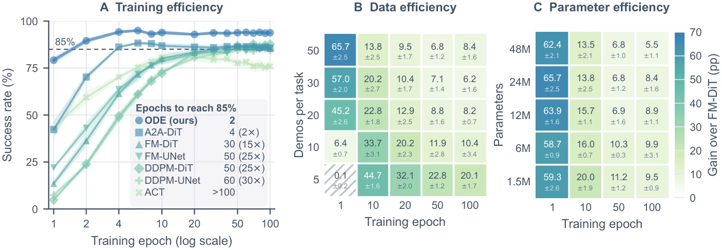
图 4:视觉运动模仿学习中的学习效率。LIBERO 上的成功率,对四个 suite 和三个随机种子取平均。(A) 训练过程中的成功率,阴影带为种子间的标准差。插图列出每种方法首次达到 85%(虚线)的 epoch 及其与 ODE 策略的比值。(B) 不同每任务示范数下,ODE 策略相对 FM-DiT 的增益(百分点);(C) 不同编码器外参数量下的同一增益。
原图注:Learning efficiency in visuomotor imitation learning. Success rates on LIBERO, averaged over the four suites and three random seeds. (A) Success rate during training, with the standard deviation over seeds as shaded bands. The inset lists the first epoch at which each method reaches 85% (dashed line) and its ratio to ODE policy. (B) Gain of ODE policy over FM-DiT in percentage points with different numbers of demonstrations per task and (C) of parameters outside the encoder.
图 4 解读
(A) 训练效率:横轴为训练 epoch(对数刻度,1–100),纵轴为成功率。ODE(深蓝圆点)第 1 个 epoch 就约 79%,第 2 个 epoch 超过 85% 虚线,之后稳定在 90% 以上;A2A-DiT 起点约 43%;FM、DDPM 系列起点在 5–20% 之间,要到 30–60 个 epoch 才达到 85%;ACT 到 100 个 epoch 仍未达到。插图中达到 85% 所需 epoch 为:ODE 2,A2A-DiT 4(2 倍),FM-DiT 30(15 倍),FM-UNet 50(25 倍),DDPM-DiT 50(25 倍),DDPM-UNet 60(30 倍),ACT >100。 (B) 数据效率:热力图行为每任务示范数(5、10、20、30、50),列为训练 epoch(1、10、20、50、100),格中为 ODE 减 FM-DiT 的成功率差(百分点)及其标准差。50 条示范、第 1 个 epoch 时差 65.7 个点;由此可推算 FM-DiT 此时约为 79.2-65.7=13.5\%,ODE 约为它的 79.2/13.5\approx5.9 倍,这正是摘要中“5.9 倍成功率”的来源。第 10 个 epoch 一列从上到下依次为 13.8、20.2、22.8、33.7、44.7,即数据越少,优势越大。5 条示范、第 1 个 epoch 的格子带斜线、差值仅 0.1,两种方法都还没学会。 (C) 参数效率:行为编码器外参数量(1.5M–48M),列同 (B)。各规模下第 1 个 epoch 的增益都在 59–66 个点,第 100 个 epoch 都在 5–10 个点,增益基本不随规模变化,说明优势来自 ODE 形式而非模型容量。
6.1.1视觉运动模仿学习
原文
Training efficiency. Against the six visuomotor baselines on LIBERO, ODE policy learns from the first epoch (Fig. 4(A)). After one epoch, it succeeds in 79.2% of the episodes, nearly twice the best baseline, while diffusion and flow policies have barely started. It passes 85% at epoch 2, an order of magnitude earlier than flow and diffusion policies, and still leads at epoch 100. Integrating over the physical time of the robot is thus far easier to learn, without trading off the final performance.
译文
训练效率。在 LIBERO 上与六种视觉运动基线相比,ODE 策略从第一个 epoch 就开始学会(图 4(A))。一个 epoch 后,它在 79.2% 的回合中成功,接近最佳基线的两倍,而扩散和流策略几乎还没有起步。它在第 2 个 epoch 就超过 85%,比流和扩散策略早一个数量级,并且到第 100 个 epoch 仍然领先。因此,在机器人的物理时间上积分要容易学得多,而且不以牺牲最终性能为代价。
解释
“接近两倍”:最佳基线是 A2A-DiT(约 43.2%),79.2/43.2\approx1.83。“早一个数量级”:FM/DDPM 需要 30–60 个 epoch,是 ODE 的 15–30 倍。为什么学得快的直觉:ODE 头每一步只需学“当前动作该往哪儿走一点”,这是一个局部、平滑、低维的映射;生成式头则要学“从高维噪声到整块动作”的复杂变换。另外 ODE 头的输入包含当前动作,等于提供了强先验“下一个动作在当前动作附近”。
原文
Data efficiency. With 5 to 50 demonstrations per task (Fig. 4(B)), ODE policy leads FM-DiT at every data scale from epoch 10 on, and the gap grows as data shrink. With 20 demonstrations per task, it reaches 87.7% at epoch 100, above FM-DiT trained on all 50 (85.4%). It matches FM-DiT with less than half of the demonstrations.
译文
数据效率。在每任务 5 到 50 条示范的范围内(图 4(B)),从第 10 个 epoch 起,ODE 策略在每个数据规模上都领先 FM-DiT,并且数据越少差距越大。在每任务 20 条示范时,它在第 100 个 epoch 达到 87.7%,高于用全部 50 条示范训练的 FM-DiT(85.4%)。它只用不到一半的示范就能达到 FM-DiT 的水平。
解释
20/50=40\%,即“不到一半”。第 100 个 epoch 时 50 条示范下 ODE 领先 8.4 个点,则 ODE 全量数据约为 85.4+8.4=93.8\%,与图 4(A) 末端一致。“从第 10 个 epoch 起”这一限定是因为 5 条示范时第 1 个 epoch 两者差距几乎为零。
原文
Parameter efficiency. Scaling the parameters outside the encoder from 1.5M to 48M (Fig. 4(C)) barely changes the gain. The smallest ODE policy (1.5M) reaches 92.5% at epoch 10, above the largest FM-DiT (48M) at any epoch (at most 87.5%). The advantage comes from the ODE formulation, not from the model capacity.
译文
参数效率。把编码器外的参数从 1.5M 扩大到 48M(图 4(C)),增益几乎不变。最小的 ODE 策略(1.5M)在第 10 个 epoch 达到 92.5%,高于最大的 FM-DiT(48M)在任何 epoch 的成绩(最高 87.5%)。优势来自 ODE 的表述,而不是模型容量。
解释
1.5M 参数比 48M 小 32 倍。这一结果对部署很有意义:动作头可以做得极小,推理延迟主要由视觉编码器决定。不过也说明在 LIBERO 这个规模上,ODE 策略并不受益于扩大动作头,至于更大规模、更难的数据上是否如此,本文没有回答。
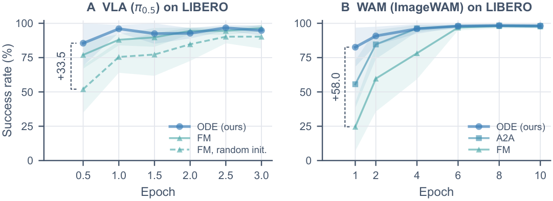
图 5:大规模模仿学习中的学习效率。ODE 头(本文)、原始流匹配头(FM)以及 (B) 中的 A2A 头在 LIBERO 上的成功率,单个种子。(A) \pi_{0.5} VLA(每任务 10 个回合),FM 专家用 \pi_{0.5} 初始化(实线)或随机初始化(虚线)。(B) ImageWAM(每任务 25 个回合)。括号标出 (A) 中相对随机初始化 FM 专家、(B) 中相对原始动作头的增益,阴影带为四个 suite 之间的标准差。各 suite 的结果见附录 B.4 和 B.5。
原图注:Learning efficiency in imitation learning at scale. Success rate on LIBERO of the ODE head (ours), the original flow matching head (FM), and an A2A head in (B), one seed. (A) The \pi_{0.5} VLA (10 episodes per task), with the FM expert initialized from \pi_{0.5} (solid) or randomly (dashed). (B) ImageWAM (25 episodes per task). Brackets mark the gain over the randomly initialized FM expert in (A) and over the original head in (B), and shaded bands the standard deviation over the four suites. Per-suite results are given in Appendix B.4 and B.5.
图 5 解读
(A) \pi_{0.5}:横轴为 epoch(0.5–3),纵轴为成功率。ODE(深蓝圆点)在 0.5 个 epoch 时约 85%,第 1 个 epoch 约 96%;预训练初始化的 FM(实线三角)在 0.5、1 个 epoch 时约 77%、88%;随机初始化的 FM-R(虚线)约 52%、75.5%。括号 +33.5 标在 0.5 个 epoch 处,是 ODE 相对 FM-R 的增益。到第 2 个 epoch 后 ODE 与预训练 FM 持平,都在 93–97% 之间。 (B) ImageWAM:横轴为 epoch(1–10)。第 1 个 epoch 时 ODE 82.6%、A2A 约 55%、FM 24.6%(括号 +58.0);第 2 个 epoch 时 FM 约 60%;第 6 个 epoch 起三者都接近 98%。 评测规模提醒:这两组实验只有一个种子,(A) 每任务只评测 10 个回合(每 suite 100 次),(B) 每任务 25 个回合,统计误差比图 4 大。阴影带是四个 suite 之间的差异,不是种子间的方差。
6.1.2大规模模仿学习
原文
To test whether the gain carries over to large pretrained models, we replace the action expert of \pi_{0.5} (Physical Intelligence et al., 2025) by a randomly initialized ODE head with about 3% of its parameters (Fig. 5(A)). Without any pretrained action weights, it leads both FM experts early in training, with 96.0% after one epoch against 75.5% for the randomly initialized one, and the pretrained expert catches up only from the second epoch on.
译文
为了检验这种增益能否延续到大型预训练模型,我们把 \pi_{0.5}(Physical Intelligence et al., 2025)的动作专家替换为一个随机初始化的 ODE 头,其参数量约为原动作专家的 3%(图 5(A))。在没有任何预训练动作权重的情况下,它在训练早期领先两种 FM 专家:一个 epoch 后为 96.0%,而随机初始化的 FM 专家为 75.5%;预训练的专家直到第二个 epoch 起才追上。
解释
13.7/430\approx3.2\%,与“约 3%”一致。口径提醒:引言中写的是“96.0% 对其流匹配专家的 75.5%”,没有说明 75.5% 是随机初始化的版本;按图 5(A),预训练的 FM 专家在第 1 个 epoch 时约为 88%,ODE 领先约 8 个点而非 20 个点。这里的正文表述是准确的,引言则容易让人高估差距。
原文
In ImageWAM, which has 4.5B trainable parameters (Fig. 5(B)), the ODE head succeeds in 82.6% after one epoch, against 24.6% for the original head, with A2A (Zuo et al., 2026) in between, and all three converge from epoch 6 on. ODE policy thus keeps its learning efficiency in large pretrained models, where the action head is only a small part of the network.
译文
在具有 4.5B 可训练参数的 ImageWAM 中(图 5(B)),ODE 头一个 epoch 后的成功率为 82.6%,而原始动作头为 24.6%,A2A(Zuo et al., 2026)介于两者之间;从第 6 个 epoch 起三者趋于一致。因此,在动作头只占网络很小一部分的大型预训练模型中,ODE 策略仍然保持了学习效率。
解释
82.6-24.6=58.0,与图中括号一致。WAM(世界动作模型)同时预测未来画面和动作,其原始动作头也是流匹配。结论的边界:在大模型中 ODE 头的优势体现为收敛更快(省几个 epoch 的算力),最终成绩三者相同。对于需要反复微调大模型的场景,这仍有实际价值。
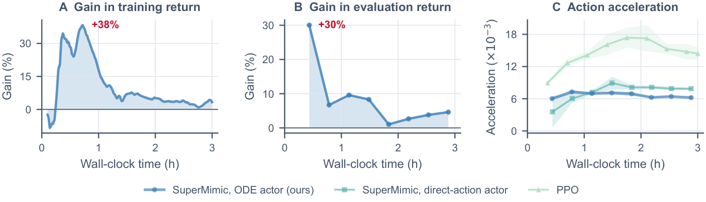
图 6:强化学习中的学习效率。在用 G1 人形机器人跟踪 40 段 LAFAN1 片段的任务上,ODE 执行器与 SuperMimic 的直接动作执行器及 PPO 的比较,横轴为单张 GPU 上的实际训练时间。(A) ODE 执行器在训练回报上的增益,(B) 在全部片段上归一化评测回报的增益,其中摔倒之后的步计为零,两者都基于三个随机种子的均值。(C) 所执行动作的加速度(越低越平滑),为三个随机种子的均值和标准差。在 0.4 小时时,直接动作执行器几乎还不会动。
原图注:Learning efficiency in reinforcement learning. The ODE actor vs. the direct-action actor of SuperMimic and PPO on tracking the 40 LAFAN1 clips with a G1 humanoid, over wall-clock time on one GPU. (A) Gain of the ODE actor in the training return and (B) in the normalized evaluation return on all clips, where the steps after a fall count as zero, both from the means over three random seeds. (C) Acceleration of the executed actions (lower is smoother), mean and standard deviation over three random seeds. At 0.4 hours, the direct-action actor still barely moves.
图 6 解读
(A) 横轴为训练时间(0–3 小时),纵轴为 ODE 执行器相对直接动作执行器的训练回报增益(%)。最初约 0.2 小时内增益为负(ODE 略慢),随后迅速上升,在约 0.75 小时达到峰值 +38\%(图中标注;正文为 37%),之后逐渐收窄,3 小时时约 +3\%。 (B) 评测回报增益:0.4 小时时 +30\%,之后在 1–10% 之间波动,最终约 +5\%。 (C) 动作加速度(\times10^{-3}):ODE(深蓝)始终在约 6–7 之间;直接动作执行器(青色)从约 3.5 升到约 8;PPO(浅绿)在 9–17 之间,明显最抖。0.4 小时时直接动作执行器的加速度反而最低,因为它“几乎还不会动”。 要点:ODE 的优势主要在训练前期,最终差距较小;在平滑度上,ODE 从 1 小时以后稳定低于直接动作执行器。
6.1.3强化学习
原文
We finally replace the actor of SuperMimic and keep its world model, critic, rewards, and hyperparameters (Fig. 6), and train PPO for the same time as a reference without a world model. The ODE actor pulls ahead early. Its training return is 37% higher after 0.75 hours (0.630\pm0.007 against 0.460\pm0.008), and its return on all 40 clips is 30% higher after 0.4 hours and stays ahead until the end (0.885\pm0.007 against 0.845\pm0.009), while PPO reaches only 0.452\pm0.021 after 3 hours (comparison with PPO in Fig. S4).
译文
最后,我们替换 SuperMimic 的执行器,而保留其世界模型、评论家、奖励和超参数(图 6),并在同样的时间内训练 PPO 作为不使用世界模型的参照。ODE 执行器很早就领先。它在 0.75 小时后的训练回报高 37%(0.630\pm0.007 对 0.460\pm0.008),在全部 40 个片段上的回报在 0.4 小时后高 30%,并一直领先到结束(0.885\pm0.007 对 0.845\pm0.009),而 PPO 在 3 小时后只达到 0.452\pm0.021(与 PPO 的比较见图 S4)。
解释
核对:0.630/0.460=1.370,即高 37%;0.885/0.845=1.047,最终高 4.7%。所以“一直领先到结束”属实,但最终差距只有约 5%,比早期的 30–37% 小得多。PPO 3 小时只有 0.452,约为 SuperMimic 的一半,这复现了 SuperMimic 论文的核心结论(可微分世界模型比无模型 RL 高效得多)。
原文
This likely stems from the gradient path along the chain of actions (Section 4.5). The gradient norm with respect to the first imagined action, relative to the last one, is about 0.57 for the direct-action actor and 1.0 to 1.1 for the ODE actor, so early actions receive a stronger learning signal. ODE policy further speeds up an already efficient RL method without any change to its algorithm.
译文
这很可能源于沿动作链的梯度路径(第 4.5 节)。相对于最后一个想象动作,对第一个想象动作的梯度范数在直接动作执行器中约为 0.57,在 ODE 执行器中为 1.0 到 1.1,因此较早的动作获得了更强的学习信号。ODE 策略无需改动算法,就进一步加快了一个本已高效的 RL 方法。
解释
这一测量支持第 4.5 节的理论分析:在 32 步想象推演中,直接动作执行器传到第一步的梯度只剩约 57%,而 ODE 执行器基本不衰减(比值约 1)。作者用“很可能”一词,表明这是相关性证据而非严格的因果证明。对熟悉 SuperMimic 的读者来说,这相当于给它的执行器加了一条“动作残差连接”。
6.2执行质量
原文
We next examine how fast ODE policy generates actions and how smoothly the robot executes them.
译文
接下来我们考察 ODE 策略生成动作的速度,以及机器人执行这些动作的平滑程度。
解释
两个指标:推理时间(毫秒/动作块)和平滑度(加加速度 jerk,越低越平滑)。
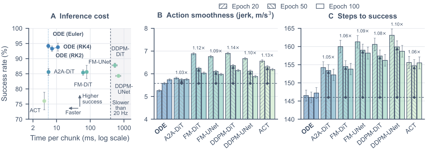
图 7:推理成本与动作平滑度。LIBERO 上的结果。(A) 第 100 个 epoch 时,每个 8 动作块的推理时间与成功率的关系,阴影区域超出 20 Hz 下 8 个控制步的 400 ms 预算。ODE 策略分别给出 RK4、RK2 和欧拉(点线)的结果。误差棒分别表示单个种子成功回合上时间的标准差,以及三个随机种子上成功率的标准差。(B) 末端位置的均方根加加速度和 (C) 完成任务所需的控制步数,统计成功回合,分别在第 20、50、100 个 epoch(以阴影区分),误差为三个随机种子所有回合的标准误。虚线标出 ODE 策略在第 50 个 epoch 的值,箭头给出各基线与之的比值(越低越好)。
原图注:Inference cost and action smoothness. Results on LIBERO. (A) Inference time per chunk of 8 actions vs. success rate at epoch 100, where the shaded region exceeds the 400 ms budget of 8 control steps at 20 Hz. ODE policy is shown with RK4, RK2, and Euler (dotted line). Error bars show the standard deviation of the time over successful episodes of one seed and of the success rate over three random seeds. (B) RMS jerk of the end-effector position and (C) control steps to complete a task over the successful episodes at epochs 20, 50, and 100 (hatching), with the standard error over the episodes of three random seeds. The dashed line marks ODE policy at epoch 50, and arrows give the ratio of each baseline to it (lower is better).
图 7 解读
(A) 横轴为每块推理时间(毫秒,对数刻度),纵轴为成功率,越靠左上越好。ODE 三种求解器都在 94% 左右,欧拉约 5.7 毫秒、RK2 约 7 毫秒、RK4 约 10 毫秒;A2A-DiT 约 5 毫秒、85.5%;FM-DiT 约 60 毫秒、85.5%;FM-UNet 约 75 毫秒;DDPM-DiT 和 DDPM-UNet 约 550–600 毫秒,落在右侧灰色区域(超出 20 Hz 控制的 400 毫秒预算);ACT 约 4 毫秒但只有约 76%。 (B) 加加速度(jerk,位置对时间的三阶导数,单位 m/s^3):ODE 约 5.3–5.8,各基线约 5.8–6.9。箭头上方的比值是各基线在第 50 个 epoch 与 ODE 的比:A2A-DiT 1.03 倍,FM-DiT 1.12 倍,FM-UNet 1.09 倍,DDPM-DiT 1.14 倍,DDPM-UNet 1.10 倍,ACT 1.13 倍。值得注意,ODE 的 jerk 随训练从约 5.3 略升至约 5.8,而多数基线随训练下降,两者差距在后期缩小。 (C) 完成任务的控制步数:ODE 约 146 步,各基线约 152–163 步,比值 1.05–1.10 倍。 解读:平滑度的优势存在但幅度不大(3–14%);速度上,ODE 与单次前向的 A2A、ACT 同档,比 FM 快一个数量级,比 DDPM 快两个数量级。
原文
Inference cost. Since the solver barely changes the success rate (Fig. 16(C)), we compare with ODE policy using Euler (Fig. 7(A)). It generates a chunk of 8 actions in 5.7 ms, as fast as A2A-DiT, 10.8 times faster than FM-DiT, and about 100 times faster than DDPM, which exceeds the budget of a 20 Hz controller. Only ACT is slightly faster, at a much lower success rate. Even with RK4, it stays several times faster than FM-DiT, and the ranking holds on an idle GPU (Table S1). ODE policy thus combines the speed of single-pass policies with a higher success rate than generative ones.
译文
推理成本。由于求解器几乎不改变成功率(图 16(C)),我们用采用欧拉法的 ODE 策略进行比较(图 7(A))。它生成一个 8 动作块只需 5.7 ms,与 A2A-DiT 一样快,比 FM-DiT 快 10.8 倍,比 DDPM 快约 100 倍,而 DDPM 超出了 20 Hz 控制器的时间预算。只有 ACT 略快,但成功率低得多。即使使用 RK4,它仍比 FM-DiT 快数倍,并且这一排序在空闲 GPU 上同样成立(表 S1)。因此,ODE 策略兼具单次前向策略的速度和比生成式策略更高的成功率。
解释
5.7\times10.8\approx62 毫秒,即 FM-DiT 每块约 62 毫秒,与图 7(A) 读数一致。口径注意:第 5 节说主实验的默认设置是 RK4,而这里的“10.8 倍”是用欧拉法测的;RK4 约 10 毫秒,相对 FM-DiT 约快 6 倍。作者的理由是求解器几乎不影响成功率,因此部署时可以选欧拉。摘要中的“快 10.8 倍”即来自这里。“空闲 GPU”是为了排除评测时 GPU 被仿真器等占用造成的计时偏差。
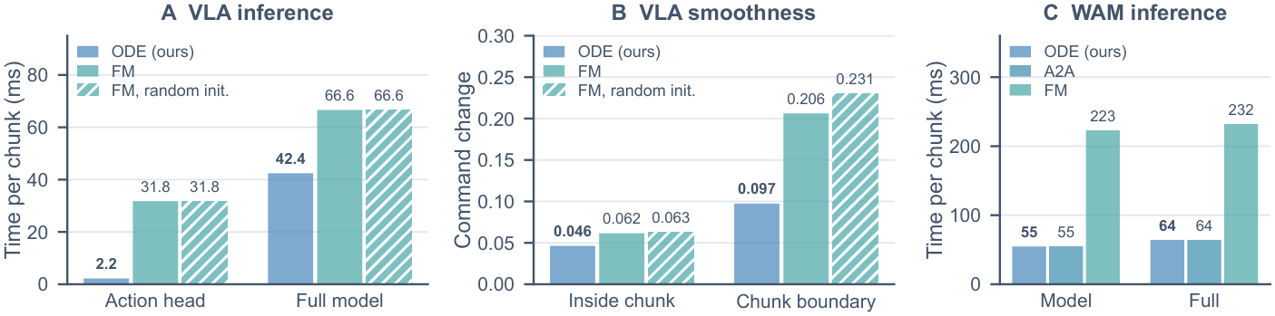
图 8:大规模模型中的推理成本与动作平滑度。LIBERO 上单个种子的结果。(A) 第 3 个 epoch 时 \pi_{0.5} 中每个 8 动作块的推理时间,分别给出动作头和完整模型,在单张 A100 GPU 上以 batch size 1 测得。(B) \pi_{0.5} 中归一化位置指令在动作块内部以及新动作块第一步的平均变化量。(C) 在缓存文本特征的情况下,ImageWAM 每个动作块的推理时间,分别给出模型和完整的本地流水线。带斜线的柱表示随机初始化的动作头。
原图注:Inference cost and action smoothness at scale. Results on LIBERO with one seed. (A) Inference time per chunk of 8 actions in \pi_{0.5} at epoch 3, for the action head and for the full model, on one A100 GPU with batch size 1. (B) Mean change of the normalized position command inside chunks and at the first step of a new chunk in \pi_{0.5}. (C) Inference time per chunk in ImageWAM with cached text features, for the model and for the full local pipeline. Hatched bars mark randomly initialized action heads.
图 8 解读
(A) \pi_{0.5} 推理时间:动作头 ODE 2.2 毫秒、FM 31.8 毫秒(随机初始化的 FM 相同);完整模型 ODE 42.4 毫秒、FM 66.6 毫秒。 (B) \pi_{0.5} 指令变化量:动作块内部相邻两步的平均变化 ODE 0.046、FM 0.062、FM-R 0.063;块边界处 ODE 0.097、FM 0.206、FM-R 0.231。 (C) ImageWAM 推理时间:模型部分 ODE 55、A2A 55、FM 223 毫秒;完整流水线 64、64、232 毫秒。 核对与解读:31.8/2.2\approx14.5,即正文“约 14 倍”;(66.6-42.4)/66.6\approx36\%,即“节省约三分之一”;0.097/0.206\approx0.47,即“约一半”;223/55\approx4.1,即“约四倍”。值得注意:ODE 在块边界的变化(0.097)仍约为块内(0.046)的两倍,说明块边界并非完全“无缝”。原文未解释,一个可能的原因是:位置指令本身从上一块终点接续,但条件 \mathbf z_t 刷新后向量场方向会突变,使边界处的单步变化(即速度)较大。与 FM 相比它已明显改善,但“结构上连续”指的是位置连续,而非速度连续。
原文
Inference cost at scale. In \pi_{0.5}, the ODE head reads the condition once per chunk and runs about 14 times faster than the FM expert with 10 denoising steps, which also saves about a third of the time of the full model (Fig. 8(A)). Its commands also change about half as much at chunk boundaries (Fig. 8(B)). In ImageWAM, the action transformer runs once per chunk and a small vector field carries out the integration, whereas the original head runs the transformer at each of its 10 denoising steps. This cuts the time per chunk about fourfold, as fast as A2A (Fig. 8(C)). Moreover, each action of ODE policy can be sent to the controller as soon as it is integrated (Section 4.3), whereas the baselines must first generate the whole chunk.
译文
大规模模型中的推理成本。在 \pi_{0.5} 中,ODE 头每个动作块读取一次条件,运行速度约为使用 10 步去噪的 FM 专家的 14 倍,这也为完整模型节省了约三分之一的时间(图 8(A))。它的指令在动作块边界处的变化量也只有约一半(图 8(B))。在 ImageWAM 中,动作 Transformer 每个动作块运行一次,由一个小型向量场完成积分,而原始动作头在 10 步去噪的每一步都要运行该 Transformer。这使每个动作块的时间缩短约四倍,与 A2A 一样快(图 8(C))。此外,ODE 策略的每个动作一经积分就可以发送给控制器(第 4.3 节),而基线必须先生成整个动作块。
解释
在大模型中,动作头加速对整体延迟的影响取决于它占比多大:\pi_{0.5} 中 VLM 主干约 40 毫秒占大头,所以动作头快 14 倍,整体只快约 36%;ImageWAM 的原始动作头本身很重(每步都跑 Transformer),所以整体快 4 倍。这提示:动作头越重的模型,换成 ODE 头的收益越大。
原文
Action smoothness. Over the successful episodes, ODE policy has the lowest end-effector jerk at every checkpoint and finishes tasks in fewer control steps than all baselines (Fig. 7(B, C)). In RL, the actions of the ODE actor accelerate 21% less than those of the direct-action actor and less than half as much as PPO after 3 hours (Fig. 6(C)). Since integration links consecutive actions and seamless chunking links the chunks (Section 8), the executed motion is both smoother and more efficient.
译文
动作平滑度。在成功的回合上,ODE 策略在每个检查点都有最低的末端加加速度,并且比所有基线用更少的控制步完成任务(图 7(B, C))。在 RL 中,训练 3 小时后,ODE 执行器的动作加速度比直接动作执行器低 21%,不到 PPO 的一半(图 6(C))。由于积分把相邻动作联系起来,无缝分块又把各动作块联系起来(第 8 节),执行的运动既更平滑又更高效。
解释
核对 RL 数字:图 6(C) 中 3 小时时 ODE 约 6.2、直接动作执行器约 7.9,1-6.2/7.9\approx22\%,与“低 21%”一致;PPO 约 14.3,ODE 不到其一半。“更高效”指用更少的步数完成任务(图 7(C) 中少 5–10%),平滑的运动减少了来回修正。
6.3泛化性能
原文
We then test how well ODE policy generalizes to perturbations unseen in training, as a visuomotor policy and within a VLA and a WAM.
译文
接着我们检验 ODE 策略对训练中未见过的扰动的泛化能力,分别作为视觉运动策略,以及在 VLA 和 WAM 之中。
解释
所有模型都只用原版 LIBERO 训练,然后在 LIBERO-plus 的扰动环境中直接测试。
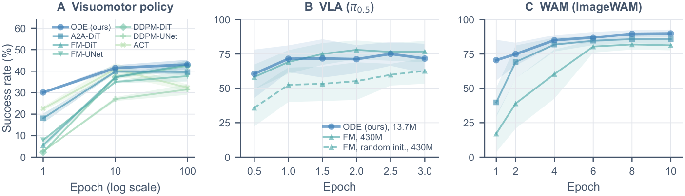
图 9:对未见扰动的泛化。LIBERO-plus 上所有扰动类型的零样本成功率。(A) 视觉运动策略,合并四个 suite,阴影带为三个随机种子的标准差。(B) \pi_{0.5} 和 (C) ImageWAM,在一组共享的 2008 个实例上测试,单个种子,阴影带为四个 suite 之间的标准差。虚线表示随机初始化的动作头,(B) 的图例给出各动作头的规模。各扰动类型的结果见图 S1 和表 S4。
原图注:Generalization to unseen perturbations. Zero-shot success rate on LIBERO-plus over all perturbation types. (A) Visuomotor policies, pooled over the four suites, with the standard deviation over three random seeds as shaded bands. (B) \pi_{0.5} and (C) ImageWAM on a shared set of 2008 instances, one seed, with the standard deviation over the four suites as shaded bands. Dashed lines mark randomly initialized action heads, and the legend of (B) gives the size of each head. Results per perturbation type are given in Fig. S1 and Table S4.
图 9 解读
(A) 视觉运动策略:横轴为 epoch(1、10、100,对数刻度)。第 1 个 epoch 时 ODE 30.1%、ACT 22.6%、A2A-DiT 约 18%、FM-UNet 约 8%、FM-DiT 约 5.6%、DDPM 系列约 2–3%;第 10 和 100 个 epoch 时各方法都升到 27–43%,ODE 与最强基线持平(约 41–43%)。由 30.1/5.6\approx5.4 可知,摘要中“泛化能力 5.4 倍”是第 1 个 epoch 时与 FM-DiT 的比值。 (B) \pi_{0.5}:横轴 0.5–3 个 epoch。ODE(13.7M)从约 60% 升到约 71–75%;预训练 FM(430M)从约 58% 升到约 75–78%;随机初始化的 FM-R(虚线)从约 36% 升到约 63%。从第 1.5 个 epoch 起,预训练 FM 的泛化成绩略高于 ODE(例如第 2 个 epoch 约 78% 对 71%)。 (C) ImageWAM:第 1 个 epoch 时 ODE 70.5%、A2A 约 40%、FM 17.1%;第 10 个 epoch 时 ODE 约 90%、A2A 约 88%、FM 约 81%,ODE 始终领先。 要点:泛化上的优势主要在训练早期;最终成绩上,ODE 在视觉运动策略中与基线持平,在 \pi_{0.5} 中略逊于预训练 FM,在 ImageWAM 中仍领先。
6.3.1视觉运动模仿学习
原文
Evaluated zero-shot on LIBERO-plus with 50 perturbed instances per type and suite (Fig. 9(A)), ODE policy leads clearly after one epoch (30.1% vs. 22.6% for ACT) and later stays on par with the strongest baselines. Per perturbation type (Fig. S1), it leads most under sensor noise, FM-DiT and DDPM-DiT handle a changed initial robot pose better, and a changed camera defeats all methods.
译文
在 LIBERO-plus 上进行零样本评测,每种扰动类型、每个 suite 各 50 个扰动实例(图 9(A))。ODE 策略在一个 epoch 后明显领先(30.1% 对 ACT 的 22.6%),之后与最强基线保持相当。按扰动类型看(图 S1),它在传感器噪声下领先最多;FM-DiT 和 DDPM-DiT 对机器人初始姿态的改变处理得更好;相机视角的改变则使所有方法都失败。
解释
每类扰动 \times 每个 suite 50 个实例;按附录 A,视觉运动策略测试 6 类扰动(不含语言),4 个 suite,共 6\times4\times50=1{,}200 个实例。按类型的发现很有意思:(1) ODE 对传感器噪声最鲁棒,与积分的平滑作用一致;(2) 对初始姿态改变,ODE 反而不如 FM-DiT 和 DDPM-DiT,可能因为 ODE 从“上一个动作”出发积分,初始姿态偏离训练分布时,起点就落在示范之外,而收缩扰动只覆盖示范附近的小范围;(3) 相机视角改变对所有方法都是致命的,这是视觉编码器的问题,与动作头无关。
6.3.2大规模模仿学习
原文
Large pretrained models generalize far better than the visuomotor policies (Fig. 9(B, C)). In \pi_{0.5}, the ODE head, with about 3% of the parameters and no pretrained action weights, leads the randomly initialized FM expert throughout training. In ImageWAM, ODE policy leads throughout training, most clearly early on (70.5% vs. 17.1% for the original head after one epoch). ODE policy reaches its robustness much earlier in training, and on a real robot it also transfers dexterous skills from public data of another lab (Section 7.3).
译文
大型预训练模型的泛化能力远好于视觉运动策略(图 9(B, C))。在 \pi_{0.5} 中,参数量约为 3%、没有预训练动作权重的 ODE 头,在整个训练过程中都领先随机初始化的 FM 专家。在 ImageWAM 中,ODE 策略在整个训练过程中都领先,早期最为明显(一个 epoch 后 70.5% 对原始动作头的 17.1%)。ODE 策略在训练中早得多地达到其鲁棒性;在真机上,它还能迁移从另一个实验室的公开数据中学到的灵巧技能(第 7.3 节)。
解释
措辞细节:\pi_{0.5} 部分只说“领先随机初始化的 FM 专家”,没有提预训练 FM。按图 9(B),预训练 FM 在 1.5 个 epoch 之后泛化成绩高于 ODE。这说明在 VLA 中,预训练的动作权重对泛化有实际贡献,ODE 头从零训练暂时无法完全弥补。大模型(60–90%)远好于小视觉运动策略(约 40%),说明泛化主要来自预训练的视觉语言表征,而不是动作头。
6.4多模态能力
原文
Since a single vector field may average distinct behaviors, we test whether ODE policy keeps the modes of the demonstrations on a 2D navigation task, where an agent passes one of four gaps in a wall to reach a goal (50 demonstrations per route) and a policy that averages the routes hits the wall. We report the success rate and the mode balance \gamma=4\min_r p_r\in[0,1], where p_r\in[0,1] is the share of successful rollouts through gap r\in\{1,\dots,4\} (Fig. 10). Randomizing the direction of the field at the start of a chunk suffices to send the integrated path into another mode, without a multi-step generative sampling process.
译文
由于单一向量场可能会平均掉不同的行为,我们在一个二维导航任务上检验 ODE 策略能否保留示范中的模式:智能体从墙上四个缺口之一穿过以到达目标(每条路线 50 条示范),而把各路线平均的策略会撞墙。我们报告成功率和模式平衡度 \gamma=4\min_r p_r\in[0,1],其中 p_r\in[0,1] 是经过缺口 r\in\{1,\dots,4\} 的成功推演所占的比例(图 10)。在动作块开始时随机化向量场的方向,就足以把积分路径送入另一个模式,而无需多步的生成式采样过程。
解释
模式平衡度 \gamma 的定义很巧妙:四条路线完全均匀时每条占 1/4,\gamma=4\times\frac14=1;只要有一条路线从未被选中,\min p_r=0,\gamma=0。例如比例为 (0.4,0.3,0.2,0.1) 时 \gamma=0.4。它只看最少被选的那条,因此对“漏掉模式”非常敏感。
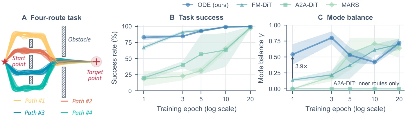
图 10:在有四条可行路线的二维导航任务上的多模态测试。(A) 智能体从起点穿过四个缺口之一到达目标点。(B) 成功率与 (C) 模式平衡度 \gamma 随训练的变化,为三个随机种子(每个 100 次推演)的均值和标准差。箭头标出一个 epoch 后 ODE 策略与 FM-DiT 的 \gamma 之比。
原图注:Multi-modal tests on a 2D navigation task with four feasible routes. (A) The agent moves from the start point through one of four gaps to the target point. (B) Success rate and (C) mode balance \gamma over training, mean and standard deviation over three random seeds with 100 rollouts each. The arrow marks the ratio of \gamma between ODE policy and FM-DiT after one epoch.
图 10 解读
(A) 左侧红星为起点,右侧圆圈为目标,中间一堵墙(灰色)有四个缺口,四种颜色的示范轨迹分别经过四个缺口(Path #1–#4)。墙后还有一块障碍物,迫使轨迹分开。 (B) 成功率:第 1 个 epoch 时 ODE 约 83%、FM-DiT 约 67%、A2A-DiT 和 MARS 约 20%;第 10 个 epoch 起 ODE 和 FM-DiT 接近 100%,MARS 和 A2A 到第 20 个 epoch 才接近 100%。 (C) 模式平衡度:ODE 第 1 个 epoch 约 0.54、第 3 个 epoch 约 0.80,之后在第 5、10 个 epoch 降到约 0.52、0.42,第 20 个 epoch 回升到约 0.72;FM-DiT 从约 0.14 逐步升到约 0.70;MARS 从 0 升到约 0.7;A2A-DiT 始终为 0(图中注“只走内侧两条路线”)。箭头“3.9\times”即 0.54/0.14。 要点:ODE 一开始就能覆盖四条路线,但其平衡度在训练中段有所下降、波动较大;FM-DiT 起步慢,但后期更稳定。摘要中“模式平衡度 3.9 倍”同样是第 1 个 epoch 的比值。
原文
With the diversity head, ODE policy takes all four routes from the first epoch (Fig. S2). Over the first five epochs, it is more balanced than FM-DiT, with 3.9 times its \gamma after one epoch, when it also succeeds more often. FM-DiT is more balanced at epoch 10, and at epoch 20 both are similarly balanced and almost always succeed. A2A-DiT with initial noise perturbation (Zuo et al., 2026) learns only the two inner routes (\gamma=0), and MARS covers all routes but learns slowly. ODE policy keeps diverse behavior while learning fast, also on a real bimanual task (Section 7.2).
译文
借助多样性头,ODE 策略从第一个 epoch 起就会走全部四条路线(图 S2)。在前五个 epoch 中,它比 FM-DiT 更平衡,一个 epoch 后其 \gamma 是 FM-DiT 的 3.9 倍,此时它的成功率也更高。到第 10 个 epoch,FM-DiT 更平衡;到第 20 个 epoch,两者平衡度相近且几乎总能成功。采用初始噪声扰动的 A2A-DiT(Zuo et al., 2026)只学会了内侧两条路线(\gamma=0),MARS 能覆盖所有路线但学得很慢。ODE 策略在快速学习的同时保持了行为多样性,在一个真实的双臂任务上也是如此(第 7.2 节)。
解释
作者如实报告了 ODE 在第 10 个 epoch 被 FM-DiT 超越。多样性头的方案(只在动作块开头采样一次方向)比完整的生成模型简单,表达能力也可能更弱,例如对需要在中途切换模式的任务,或模式之间差异更细微的情况。这个二维任务的模式非常清晰(四个分离的缺口),在更复杂的真实多模态任务上的表现需看第 7.2 节。
7真实世界结果(Real-World Results)
原文
We then deploy ODE policy on four real robots to test whether its advantages carry over to high-precision, long-horizon, deformable, multi-modal, dexterous, and loco-manipulation tasks, and finally compare the inference cost and the smoothness across the robots.
译文
接着我们把 ODE 策略部署到四台真实机器人上,检验其优势能否延续到高精度、长时程、可变形物体、多模态、灵巧操作和移动操作任务,最后比较各机器人上的推理成本和平滑度。
解释
四台机器人、14 个任务:单臂 4 个、双臂 4 个、灵巧手 4 个、人形 2 个。每个任务每种方法 20 次试验,单次试验相当于 5 个百分点。
7.1单臂机器人
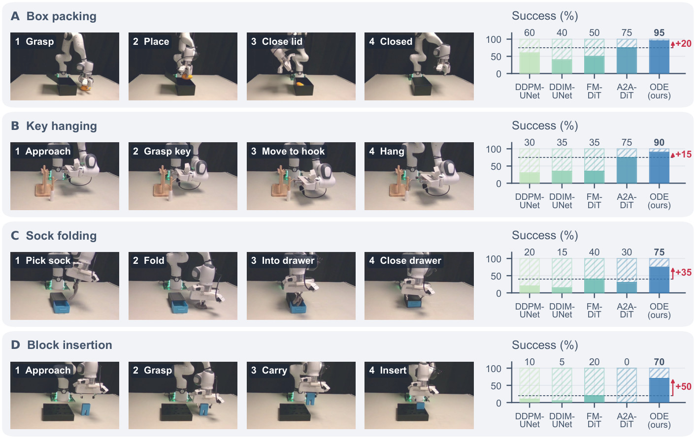
图 11:真实单臂机器人上的任务。Franka Research 3 机械臂上的 ODE 策略,每行一个任务。(A) 把芒果放进盒子并合上盖子。(B) 把钥匙挂到钥匙架上。(C) 折叠袜子并放进抽屉。(D) 把方块插进板上的孔中。右侧为 20 次试验的成功率,失败试验以斜线表示,箭头标出相对最佳基线的提升。
原图注:Tasks on a real single-arm robot. ODE policy on a Franka Research 3 arm, one row per task. (A) Putting a mango into a box and closing the lid. (B) Hanging a key on a key holder. (C) Folding a sock and putting it into a drawer. (D) Inserting a block into a hole of a board. On the right, success rates over 20 trials, with failed trials hatched and arrows from the best baseline.
图 11 解读
四行任务,每行左侧四帧展示 ODE 的执行过程,右侧柱状图依次为 DDPM-UNet、DDIM-UNet、FM-DiT、A2A-DiT、ODE 的成功率(%):(A) 装盒 60、40、50、75、95(+20);(B) 挂钥匙 30、35、35、75、90(+15);(C) 叠袜子 20、15、40、30、75(+35);(D) 插方块 10、5、20、0、70(+50)。 注意:单臂实验只训练 50 个 epoch,衡量的是早期学习效果。扩散和流匹配基线在 50 个 epoch 时可能还远未收敛(参照图 4(A),FM-DiT 在 LIBERO 上要 30 个 epoch 才达到 85%),所以这里的大幅领先部分反映了学习速度的差异。
原文
On a Franka Research 3 arm, all policies are trained on 40 demonstrations per task for only 50 epochs, to test their performance early in training. ODE policy achieves the highest success rate on all four tasks (Fig. 11), with the clearest margins in folding a sock and inserting a block (15 and 14 of 20 trials against 8 and 4 for the best baseline). A2A-DiT comes closest on the first two tasks, likely because it also generates each chunk from the previous actions, but fails all insertions.
译文
在 Franka Research 3 机械臂上,所有策略都在每任务 40 条示范上只训练 50 个 epoch,以测试训练早期的性能。ODE 策略在全部四个任务上都取得了最高成功率(图 11),在叠袜子和插方块上优势最为明显(20 次中分别成功 15 次和 14 次,而最佳基线为 8 次和 4 次)。A2A-DiT 在前两个任务上最接近,可能是因为它同样从先前的动作生成每个动作块,但它在插方块任务上全部失败。
解释
核对:75% =15/20,70% =14/20,最佳基线 40% =8/20(FM-DiT 叠袜子)、20% =4/20(FM-DiT 插方块),与图一致。A2A-DiT 在插方块上为 0,而在前两个任务上与 ODE 相差 15–20 个点,说明“从历史动作出发”这一共同点有帮助,但高精度插入需要更多。
原文
At the chunk boundaries, ODE policy also commands the lowest acceleration on every task, 3.6, 1.1, 2.5, and 2.2 rad/s^2, against 2.8 to 9.1 for A2A-DiT and 8.3 to 26.0 for the diffusion and flow matching baselines. It learns multi-stage, deformable, and high-precision tasks reliably from a few dozen demonstrations within a short training.
译文
在动作块边界处,ODE 策略在每个任务上发出的加速度指令也都是最低的,分别为 3.6、1.1、2.5 和 2.2 rad/s^2,而 A2A-DiT 为 2.8 到 9.1,扩散和流匹配基线为 8.3 到 26.0。它能在短时间训练内,从几十条示范中可靠地学会多阶段、可变形物体和高精度任务。
解释
单位 rad/s^2 是关节角加速度,衡量指令在块边界处“拐弯”有多急。扩散和流匹配基线比 ODE 高 3–10 倍,说明它们在块边界处有明显的突变。A2A-DiT 介于两者之间:它从历史动作出发生成新块,部分缓解了边界问题,但不像 ODE 那样严格接续。
7.2双臂机器人
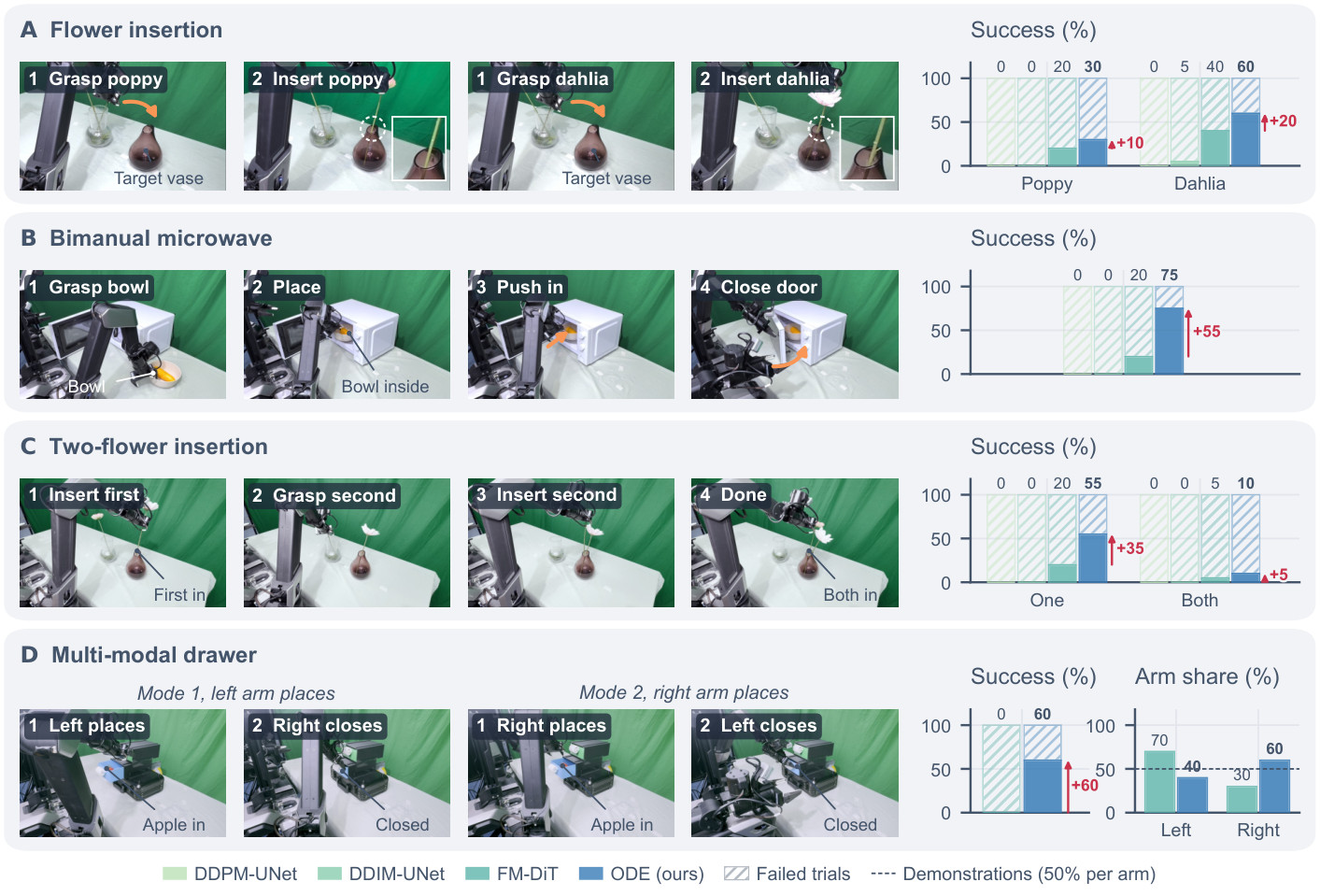
图 12:真实双臂机器人上的四个任务。Galaxea R1 Lite 上的 ODE 策略,每行一个任务。(A) 把一支罂粟花或大丽花插进花瓶的窄口(虚线圈及放大图)。(B) 把碗放进微波炉、推到里面并关上门。(C) 先后插入两支花。(D) 任一只手臂把苹果放进抽屉,另一只手臂关上抽屉,每种模式两帧。右侧为每种花或每个任务 20 次试验的成功率,失败试验以斜线表示,箭头标出相对最佳基线的提升。(D) 中旁边给出每只手臂去拿苹果的试验比例,虚线为示范中的比例。
原图注:Four tasks on a real dual-arm robot. ODE policy on the Galaxea R1 Lite, one row per task. (A) Inserting a poppy or a dahlia into the narrow opening of a vase (dashed circle and zoom). (B) Putting a bowl into a microwave, pushing it in, and closing the door. (C) Inserting two flowers one after the other. (D) Either arm puts an apple into the drawer and the other closes it, two frames per mode. On the right, success rates over 20 trials per flower or task, with failed trials hatched and arrows from the best baseline. In (D), the share of trials in which each arm goes for the apple is shown next to it, with the dashed line at the share in the demonstrations.
图 12 解读
柱状图依次为 DDPM-UNet、DDIM-UNet、FM-DiT、ODE 的成功率(%):(A) 插花:罂粟 0、0、20、30(+10),大丽花 0、5、40、60(+20);(B) 微波炉 0、0、20、75(+55);(C) 两支花:插入第一支 0、0、20、55(+35),两支都插入 0、0、5、10(+5);(D) 多模态抽屉:只比较 FM-DiT(0)和 ODE(60)。(D) 右侧“Arm share”:ODE 左臂去拿苹果 40%、右臂 60%,示范中各 50%(虚线);FM-DiT 也两只手臂都会去拿(左臂占多数),但从未成功放入。 要点:两个扩散基线在前三个任务上几乎全部失败;ODE 在长时程的微波炉任务上优势最大,但“插两支花”全部成功只有 10%,罂粟花也只有 30%,绝对成功率并不高。
原文
On the Galaxea R1 Lite, ODE policy is tested on four tasks, two of them with both arms (Fig. 12).High-precision and long-horizon tasks. In flower insertion, the thin stem must meet the narrow opening of a vase, and the long stem of the poppy amplifies small errors at the gripper. ODE policy succeeds more often than FM-DiT with both flowers (60% vs. 40% with the dahlia), likely because its motion stays smooth up to the opening. In the microwave task, learned from only 34 demonstrations, it succeeds in 75% of the trials against 20% for FM-DiT, which leaves the door open in 9 of its 16 failures, against 2 of 5 for ODE policy.
译文
在 Galaxea R1 Lite 上,ODE 策略在四个任务上接受测试,其中两个需要双臂(图 12)。高精度和长时程任务。在插花任务中,细长的花茎必须对准花瓶的窄口,罂粟花较长的茎会放大夹爪处的微小误差。ODE 策略对两种花的成功次数都多于 FM-DiT(大丽花 60% 对 40%),可能是因为它的运动直到瓶口都保持平滑。在只用 34 条示范学习的微波炉任务中,它在 75% 的试验中成功,而 FM-DiT 为 20%;FM-DiT 的 16 次失败中有 9 次没关上门,而 ODE 策略的 5 次失败中只有 2 次如此。
解释
核对:FM-DiT 20% 即 4/20 成功、16 次失败;ODE 75% 即 15/20、5 次失败,与正文一致。罂粟花茎长,夹持点到茎尖的距离大,角度误差会被杠杆放大,所以比大丽花难得多。“可能是因为运动平滑”是作者的推测,没有单独验证。
原文
Chaining two insertions into the same vase, it inserts the first flower far more often than FM-DiT (55% vs. 20%), although the second insertion, into a vase that already holds a stem, is hard for all methods. Both diffusion policies fail almost every trial of the three tasks. ODE policy thus keeps the error of each step small enough for precise and long sequences with both arms.
译文
把两次插入串联到同一个花瓶时,它插入第一支花的次数远多于 FM-DiT(55% 对 20%),尽管第二次插入(插进已有一支花茎的花瓶)对所有方法都很难。两种扩散策略在这三个任务上几乎每次都失败。因此,ODE 策略能把每一步的误差保持得足够小,以完成双臂的精确长序列操作。
解释
两支都插入:ODE 10%(2/20),FM-DiT 5%(1/20),差别只有一次试验,不具统计意义。这也是本文“在每个任务上都取得最高成功率”这一说法中最弱的一项。
原文
Multi-modal task. In the drawer task (Fig. 12(D)), one arm puts an apple into an open drawer and the other closes it, and the demonstrations assign the two roles both ways equally often. With the diversity head (Section 4.4), ODE policy takes both modes, with the left arm placing the apple in 8 of the 20 trials and the right arm in 12, and succeeds in 5 of 8 and 7 of 12, 60% in total. FM-DiT also goes for the apple with both arms but never places it. The multi-modality seen in navigation carries over to a bimanual robot.
译文
多模态任务。在抽屉任务中(图 12(D)),一只手臂把苹果放进打开的抽屉,另一只手臂把抽屉关上,示范中两种角色分配出现的次数相同。借助多样性头(第 4.4 节),ODE 策略两种模式都会采用:20 次试验中左臂放苹果 8 次、右臂放苹果 12 次,分别成功 5 次和 7 次,总计 60%。FM-DiT 也会用两只手臂去拿苹果,但从未成功放入。在导航任务中观察到的多模态能力延续到了双臂机器人上。
解释
核对:(5+7)/20=60\%。模式比例 40:60,接近示范的 50:50。这是多样性头在真机上的直接证据,与本工作区 RoboICL 译稿附录中 Fill Pen Holder 的“双臂角色切换”可以对照:后者是大模型从示范中组合角色,这里是小策略学会按比例选择角色。
7.3灵巧手
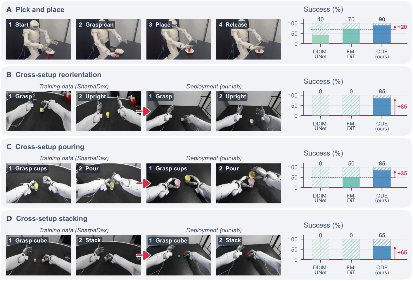
图 13:带灵巧手的真实机器人上的任务。配备 Sharpa 灵巧手的 Sharpa North 机器人上的 ODE 策略,每行一个任务。(A) 拿起罐子并放到盘子上。(B-D) 只用另一个实验室的公开示范(Sharpa Robotics, 2026)学习(左)并部署在我们实验室(右)的任务:(B) 把倒下的杯子扶正,(C) 用双手把药片从一个杯子倒进另一个杯子,(D) 把一个方块叠到另一个上。右侧为 20 次试验的成功率,失败试验以斜线表示,箭头标出相对最佳基线的提升。
原图注:Tasks on a real robot with a dexterous hand. ODE policy on the Sharpa North robot with a Sharpa hand, one row per task. (A) Picking up a can and placing it on a plate. (B-D) Tasks learned only from public demonstrations of another lab (Sharpa Robotics, 2026) (left) and deployed in our lab (right), (B) reorienting a fallen cup upright, (C) pouring pills from one cup into another with two hands, and (D) stacking one cube on another. On the right, success rates over 20 trials, with failed trials hatched and arrows from the best baseline.
图 13 解读
柱状图依次为 DDIM-UNet、FM-DiT、ODE 的成功率(%):(A) 抓放罐子 40、70、90(+20);(B) 跨场景扶杯 0、0、85(+85);(C) 跨场景倒药片 0、50、85(+35);(D) 跨场景叠方块 0、0、65(+65)。(B)–(D) 每行左两帧是 Sharpa 公司实验室的训练数据画面,右两帧是本文实验室的部署画面,可见桌面、背景和物体颜色都不同。 要点:跨场景迁移是本文最引人注目的真机结果之一,两个基线在三个跨场景任务中有两个完全失败。
原文
Pick-and-place with a dexterous hand. On a Sharpa North robot with a Sharpa dexterous hand, whose joints greatly enlarge the action space, ODE policy picks up a can and places it on a plate in 18 of 20 trials after training on 50 demonstrations, against 14 for FM-DiT and 8 for DDIM-UNet (Fig. 13(A)).
译文
灵巧手抓放。在配备 Sharpa 灵巧手的 Sharpa North 机器人上(灵巧手的关节大大扩展了动作空间),ODE 策略用 50 条示范训练后,20 次试验中有 18 次拿起罐子并放到盘子上,而 FM-DiT 为 14 次,DDIM-UNet 为 8 次(图 13(A))。
解释
五指灵巧手通常有 20 个左右的关节自由度,加上手臂,动作维度可达数十维。高维空间中,生成式方法需要从高维噪声开始去噪,难度更大;ODE 每步只学一个局部增量,维度高并不显著增加难度。
原文
Cross-setup transfer. We next train on 50 demonstrations per task from the public SharpaDex dataset (Sharpa Robotics, 2026), recorded by Sharpa in its own lab with the same robot and hand, and deploy the policies in our lab without any demonstration from our setup (Fig. 13(B-D)). In reorienting a fallen cup upright, with other cups and another background, ODE policy succeeds in 17 of 20 trials, while FM-DiT never grasps the cup and DDIM-UNet hovers above it with the hand jittering at the period of one chunk.
译文
跨场景迁移。接下来,我们在公开的 SharpaDex 数据集(Sharpa Robotics, 2026)上每任务用 50 条示范训练,这些示范由 Sharpa 公司在其自己的实验室用同型号机器人和灵巧手录制;然后在我们的实验室部署这些策略,不使用来自我们环境的任何示范(图 13(B-D))。在把倒下的杯子扶正的任务中,换用了其他杯子和另一种背景,ODE 策略 20 次中成功 17 次,而 FM-DiT 从未抓住杯子,DDIM-UNet 则悬停在杯子上方,手以一个动作块为周期抖动。
解释
“以一个动作块为周期抖动”是块边界不连续最直观的表现:每生成一个新块,手就跳一下,周而复始,始终无法稳定地下去抓。这为“块边界连续性”的重要性提供了生动的反例。跨场景迁移在机器人学习中很难,因为光照、背景、相机位置的细微差异都会影响视觉编码器;ODE 在这里的大幅领先,作者归因于其鲁棒性,但视觉编码器是共享的,差异主要来自动作头,这一点值得进一步研究。
原文
In pouring pills between two cups with two hands, using cups of other colors, it succeeds in 17 trials against 10 for FM-DiT and none for DDIM-UNet. In stacking a red cube on a green one, whereas the demonstrations use wooden cubes, it succeeds in 13 of 20 trials, while both baselines always fail. ODE policy thus carries skills across setups, consistent with its robustness to unseen perturbations in simulation (Section 6.3).
译文
在用双手把药片从一个杯子倒进另一个杯子的任务中(使用其他颜色的杯子),它成功 17 次,而 FM-DiT 为 10 次,DDIM-UNet 为 0 次。在把红色方块叠到绿色方块上的任务中(而示范使用的是木质方块),它 20 次中成功 13 次,而两个基线全部失败。因此,ODE 策略能把技能跨场景迁移,这与它在仿真中对未见扰动的鲁棒性一致(第 6.3 节)。
解释
叠方块任务中物体从木色变成红绿两色,属于外观上的分布偏移;ODE 仍有 65%。与仿真的一致性要谨慎看待:第 6.3 节中视觉运动策略在 LIBERO-plus 上最终与基线持平,只在早期领先;而这里真机跨场景是大幅领先。两者并不完全一致,真机的结果更强,可能与真机训练只到 300 个 epoch、基线尚未充分学会有关,也可能与灵巧手的高维动作空间有关。
7.4人形机器人
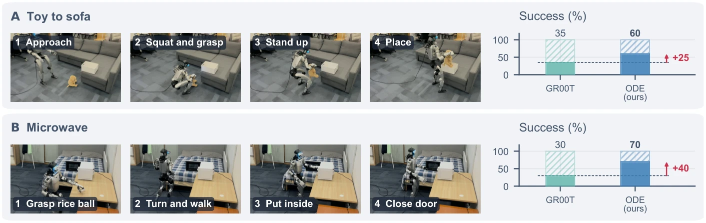
图 14:真实人形机器人上的移动操作任务。在配备 Inspire DFX 灵巧手的宇树 G1 上,ODE 策略作为 GR00T N1.7 的动作头,每行一个任务。(A) 走到地板上的玩具旁,蹲下抓起,站起来,把它放进沙发上的盒子里。(B) 从桌上拿起一个饭团,转身走到微波炉前,把饭团放进去,并关上门。右侧为 20 次试验的成功率,失败试验以斜线表示,箭头标出相对基线的提升。
原图注:Loco-manipulation tasks on a real humanoid. ODE policy as the action head of GR00T N1.7 on a Unitree G1 with Inspire DFX dexterous hands, one row per task. (A) Walking to a toy on the floor, squatting to grasp it, standing up, and placing it into a box on the sofa. (B) Grasping a rice ball from a table, turning and walking to a microwave, putting the rice ball inside, and closing the door. On the right, success rates over 20 trials, with failed trials hatched and arrows from the baseline.
图 14 解读
(A) 玩具放沙发:GR00T 原动作头 35%、ODE 60%(+25);(B) 微波炉:GR00T 30%、ODE 70%(+40)。左侧四帧分别是接近、蹲下抓取、站起、放置,以及抓饭团、转身行走、放入、关门。
原文
We finally test whether ODE policy also drives the whole body of a humanoid. On a Unitree G1 with Inspire DFX dexterous hands, it replaces the action head of GR00T N1.7 (Bjorck et al., 2025) (Fig. 14). Both tasks are long-horizon and couple walking with a precise grasp. In the toy task, the robot walks to a toy on the floor, squats to grasp it, stands up, and places it into a box on the sofa, so the legs, the torso, and the arms must move together. In the microwave task, it grasps a small rice ball from a table, turns and walks to a microwave, puts the rice ball inside, and closes the door.
译文
最后我们检验 ODE 策略能否驱动人形机器人的全身。在配备 Inspire DFX 灵巧手的宇树 G1 上,它替换 GR00T N1.7(Bjorck et al., 2025)的动作头(图 14)。两个任务都是长时程的,并把行走与精确抓取结合在一起。在玩具任务中,机器人走到地板上的玩具旁,蹲下抓起它,站起来,再把它放进沙发上的盒子里,因此腿、躯干和手臂必须协同运动。在微波炉任务中,它从桌上抓起一个小饭团,转身走到微波炉前,把饭团放进去,并关上门。
解释
这里 ODE 头是在 GR00T N1.7 上微调的一个约 5M 参数的向量场(第 5 节),欧拉法、H=16。人形机器人的“动作”通常包括上肢关节目标和下肢的行走指令(速度、高度等),由底层的运动控制器执行。
原文
Trained on 90 demonstrations per task for 90 epochs, ODE policy succeeds in 60% and 70% of 20 trials, against 35% and 30% for the original head of GR00T. The vector field thus also carries whole-body loco-manipulation, where small errors of the stance and the grasp likely accumulate over the long task.
译文
每个任务用 90 条示范训练 90 个 epoch 后,ODE 策略在 20 次试验中的成功率为 60% 和 70%,而 GR00T 的原始动作头为 35% 和 30%。因此,向量场也能驱动全身移动操作;在这类任务中,站姿和抓取的微小误差很可能在长任务中不断累积。
解释
成功率翻倍左右。与 \pi_{0.5} 中的情况相比,GR00T 的原动作头很可能沿用其预训练权重(原文未明说),而 ODE 头是新加的约 5M 参数向量场,因此对 ODE 而言同样是“以小搏大”。不过只有两个任务、各 20 次试验,结论的普适性有限。
7.5推理成本与平滑度
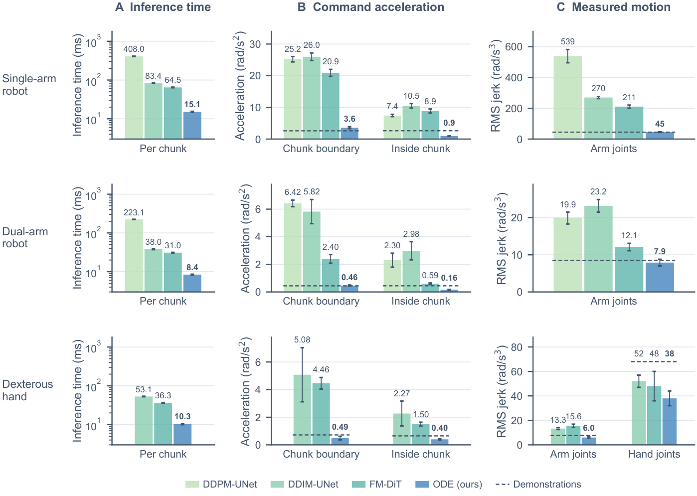
图 15:真机上的推理成本与平滑度。从上到下依次为装盒、微波炉和抓罐子任务。(A) 分别在一张 RTX 5080、RTX 5090 和 RTX 4090 上每个动作块的推理时间,对数刻度。(B) 动作块边界处和动作块内部关节指令的加速度。(C) 实测关节运动的均方根加加速度。为各回合的均值和标准差(单臂机器人只统计成功回合),虚线为示范的数值。
原图注:Inference cost and smoothness on real robots. The close-box, microwave, and can tasks (top to bottom). (A) Inference time per chunk on one RTX 5080, RTX 5090, and RTX 4090, in log scale. (B) Acceleration of the joint commands at chunk boundaries and inside chunks. (C) RMS jerk of the measured joint motion. Mean and standard deviation over episodes (successful ones on the single-arm robot), with the demonstrations as dashed lines.
图 15 解读
三行对应单臂(装盒)、双臂(微波炉)、灵巧手(抓罐子)。柱子依次为 DDPM-UNet、DDIM-UNet、FM-DiT、ODE(灵巧手没有 DDPM)。 (A) 每块推理时间(毫秒):单臂 408.0、83.4、64.5、15.1;双臂 223.1、38.0、31.0、8.4;灵巧手 53.1(DDIM)、36.3(FM)、10.3。最大倍数 408/15.1\approx27,最小倍数 36.3/10.3\approx3.5,即正文“快 3.5 到 27 倍”。 (B) 指令加速度(rad/s^2):单臂块边界 25.2、26.0、20.9、3.6,块内 7.4、10.5、8.9、0.9;双臂块边界 6.42、5.82、2.40、0.46,块内 2.30、2.98、0.59、0.16;灵巧手块边界 5.08、4.46、0.49,块内 2.27、1.50、0.40。虚线为示范的加速度。 (C) 实测关节加加速度(rad/s^3):单臂 539、270、211、45;双臂 19.9、23.2、12.1、7.9;灵巧手手臂关节 13.3、15.6、6.0,手指关节 52、48、38。示范的值(虚线)在单臂约 45、双臂约 8.5、手指约 68。 要点:ODE 在块边界的加速度比基线低一个数量级,且与示范相当或更低;“比人类示范更平滑”在双臂和灵巧手上成立,在单臂上与示范持平。
原文
On one task of each of the first three robots, the close-box, microwave, and can tasks (Fig. 15), ODE policy generates a chunk 3.5 to 27 times faster than the diffusion and flow matching baselines, even with RK4. Since each chunk continues from the end of the previous one, its command acceleration at chunk boundaries stays at or below that of the demonstrations on the dual-arm robot and the hand and close to it on the single-arm robot, whereas the baselines reach several times that of the demonstrations.
译文
在前三台机器人各选一个任务,即装盒、微波炉和抓罐子任务上(图 15),即使使用 RK4,ODE 策略生成一个动作块也比扩散和流匹配基线快 3.5 到 27 倍。由于每个动作块都从前一块的末端接续,它在动作块边界处的指令加速度在双臂机器人和灵巧手上不超过示范的水平,在单臂机器人上则接近示范,而基线达到示范的数倍。
解释
“即使使用 RK4”:真机默认用 RK4(第 5 节),每步 4 次网络计算,仍然快得多。在单臂上 ODE 的块边界加速度 3.6 略高于示范(约 2.7),所以说“接近”。基线在单臂上达到 20–26,是示范的 8–10 倍。
原文
The measured jerk of its arm and hand joints also matches or undercuts the demonstrations, while the arm jerk of the baselines exceeds them by up to an order of magnitude. A2A-DiT, which also starts from the previous actions, moves about as smoothly on the single-arm robot (39 rad/s^3) and generates a chunk faster (8.6 ms), but accelerates more at chunk boundaries (9.1 against 3.6 rad/s^2). Appendix B.6 reports the same measures on the cup and pill tasks.
译文
它的手臂和手部关节的实测加加速度也与示范相当或更低,而基线的手臂加加速度最多超出示范一个数量级。同样从先前动作出发的 A2A-DiT 在单臂机器人上运动得差不多一样平滑(39 rad/s^3),生成动作块也更快(8.6 ms),但在动作块边界处加速度更大(9.1 对 3.6 rad/s^2)。附录 B.6 报告了杯子和药片任务上的同样指标。
解释
公允之处:作者如实指出 A2A-DiT 在单臂上比 ODE 更快(8.6 对 15.1 毫秒)、实测加加速度也略低(39 对 45),只是块边界加速度更大。A2A-DiT 未出现在图 15 中,这些数字只在正文给出。单臂上 DDPM-UNet 的实测加加速度 539 约为示范的 12 倍,即“超出一个数量级”。
8消融研究(Ablation Studies)
原文
We ablate the design choices of ODE policy one at a time with all other settings fixed, namely the chunk length and the solver (Fig. 16), the contractive perturbation, seamless chunking, and the placement of the proprioception (Fig. 17), and the number of components of the diversity head (Fig. 18). The diversity head at inference and the architecture of the vector field are ablated in Appendix B.8.
译文
我们在固定其他所有设置的情况下,每次只改变一个设计选择,对 ODE 策略进行消融:动作块长度和求解器(图 16),收缩扰动、无缝分块以及本体感知的输入位置(图 17),以及多样性头的分量数(图 18)。推理时的多样性头和向量场的网络结构在附录 B.8 中进行消融。
解释
六个消融对应方法中的六个设计点。读图时注意每个设计在早期(第 1 个 epoch)和后期的影响往往不同:很多设计主要影响学习速度。
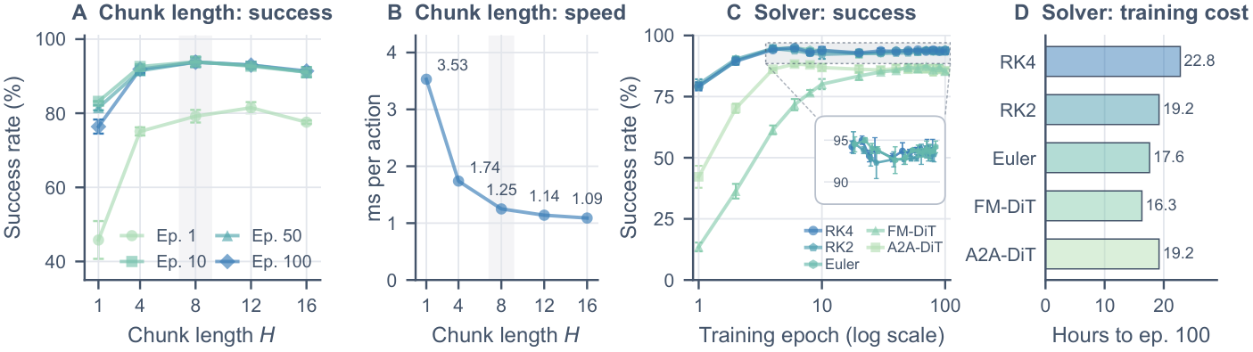
图 16:动作块长度与积分求解器的消融。ODE 策略在 LIBERO 上的结果,对四个 suite 取平均。(A) 第 1、10、50、100 个 epoch 时成功率随动作块长度 H 的变化。(B) 第 100 个 epoch 时在一张空闲 GPU 上每个动作的推理时间,默认 H=8 以灰色标出。(C) 三种求解器在训练过程中的成功率,以 FM-DiT 和 A2A-DiT 为参照,插图放大显示求解器之间的差别。(D) 训练到第 100 个 epoch 的时间(每次运行一张 RTX 4090,八次运行并行)。三个随机种子的均值和标准差(H=16 只有两个,因为第三个种子的训练发散了)。
原图注:Ablations of the chunk length and the integration solver. Results of ODE policy on LIBERO, averaged over the four suites. (A) Success rate with chunk length H at epochs 1, 10, 50, and 100. (B) Inference time per action at epoch 100 on one idle GPU, with the default H=8 in gray. (C) Success rate during training with three solvers, with FM-DiT and A2A-DiT as references and an inset on the solvers. (D) Training time to epoch 100 (one RTX 4090 per run, eight runs in parallel). Mean and standard deviation over three random seeds (two for H=16, as training with the third diverged).
图 16 解读
(A) 横轴为 H\in\{1,4,8,12,16\}。H=1 时第 100 个 epoch 只有 76.4%,第 1 个 epoch 仅约 45%;H\ge4 时各 epoch 都在 91% 以上(第 1 个 epoch 约 80%);H=8 略好。 (B) 每个动作的推理时间:H=1,4,8,12,16 分别为 3.53、1.74、1.25、1.14、1.09 毫秒。H 越大,视觉编码器的开销被越多动作分摊。 (C) RK4、RK2、欧拉三条曲线几乎重合(插图显示后期都在 93–95% 之间),都高于 FM-DiT 和 A2A-DiT。 (D) 训练到第 100 个 epoch 的小时数:RK4 22.8、RK2 19.2、欧拉 17.6、FM-DiT 16.3、A2A-DiT 19.2。注意:主实验默认的 RK4 比 FM-DiT 多花约 40% 的训练时间,正文“训练时间与 FM-DiT 相当”说的是欧拉法。 稳定性:H=16 的第三个种子训练发散,正文说 H\ge12 时有“偶发的损失尖峰”,较长动作块下反向传播要穿过更多求解步,可能导致梯度不稳定。
原文
Chunk length. With chunk length H=1 in training and execution (Fig. 16(A, B)), the policy reaches only 76.4% at epoch 100 and is the slowest per action, since the encoder runs at every step. From H=4 on, the success rate stays above 91% (best at the default H=8), while the time per action keeps falling, although training shows occasional loss spikes for H\ge12. Consistent with the finding that chunking mitigates the compounding errors of behavioral cloning (Lazzati et al., 2026; Park, 2026), chunking is essential, and H=8 balances success rate and inference time.
译文
动作块长度。在训练和执行中都取动作块长度 H=1 时(图 16(A, B)),策略在第 100 个 epoch 只达到 76.4%,并且每个动作最慢,因为编码器每一步都要运行。从 H=4 开始,成功率保持在 91% 以上(默认的 H=8 最好),每个动作的时间持续下降,不过在 H\ge12 时训练会出现偶发的损失尖峰。与“分块能缓解行为克隆中的复合误差”这一发现(Lazzati et al., 2026; Park, 2026)一致,分块是必不可少的,H=8 在成功率和推理时间之间取得平衡。
解释
H=1 时 ODE 策略退化为“每步观测一次、走一步欧拉/RK4”,此时它与 RL 中的形式相同,已经没有“块内连续积分”的优势,性能大幅下降。这说明ODE 策略的优势与分块密切相关,单靠“动作残差”式的结构是不够的。
原文
Integration solver. Replacing RK4 with RK2 or Euler changes the success rate at epoch 100 by less than one point, within the variation across seeds, and all three stay above FM-DiT and A2A-DiT throughout training (Fig. 16(C)). The cheaper solvers shorten both training and inference (Fig. 16(D)). With Euler, training takes about as long as for FM-DiT and less than for A2A-DiT, so the gain does not come from a longer training. Since even Euler applies the same vector field at every step, the performance comes from the ODE formulation, not from an accurate solver.
译文
积分求解器。把 RK4 换成 RK2 或欧拉法,第 100 个 epoch 的成功率变化不到一个百分点,处于种子间波动范围之内,并且三者在整个训练过程中都高于 FM-DiT 和 A2A-DiT(图 16(C))。更廉价的求解器同时缩短了训练和推理时间(图 16(D))。使用欧拉法时,训练时间与 FM-DiT 大致相当,且少于 A2A-DiT,因此增益并非来自更长的训练。由于即使是欧拉法也在每一步应用同一个向量场,性能来自 ODE 的表述,而不是来自精确的求解器。
解释
欧拉法相当于“下一个动作 = 当前动作 + 网络输出”,与 RL 中的公式 (11) 完全相同。这表明 ODE 策略的本质可以理解为一个以当前动作为输入、在块内自回归地输出动作增量的小网络,“ODE”和“积分”的数学语言更多是提供了理解框架和设计灵感(如收缩扰动、任意频率)。
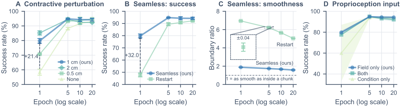
图 17:收缩扰动、无缝分块和本体感知的消融。ODE 策略在 LIBERO 上的结果,对四个 suite 取平均(每任务 10 个回合)。(A) 不使用收缩扰动以及使用三种幅度的收缩扰动。(B, C) 无缝分块与“每个动作块从实测状态重新开始”的对比,分别为成功率和边界比(动作块第一步的指令变化除以块内的指令变化)。(D) 本体感知输入到向量场、同时输入到条件和向量场,或只输入到条件。(A) 和 (B) 中的箭头标出一个 epoch 后的差距。三个随机种子的均值和标准差,(C) 中的插图显示最大的标准差。
原图注:Ablations of the contractive perturbation, seamless chunking, and proprioception. Results of ODE policy on LIBERO, averaged over the four suites (10 episodes per task). (A) Without the contractive perturbation and with three magnitudes of it. (B, C) Seamless chunking vs. restarting each chunk from the measured state, success rate and boundary ratio (command change at the first step of a chunk divided by that inside chunks). (D) Proprioception fed to the vector field, to both the condition and the field, or to the condition. Arrows in (A) and (B) mark the gap after one epoch. Mean and standard deviation over three random seeds, with an inset in (C) on the largest standard deviation.
图 17 解读
四幅子图的横轴都是 epoch(1、5、10、20,对数刻度)。 (A) 收缩扰动:扰动幅度 1 厘米(默认)第 1 个 epoch 79.8%,2 厘米约 85%,0.5 厘米约 71%,不加扰动 58.4%(箭头 +21.4);第 5 个 epoch 起都在 88–95% 之间,2 厘米略低于其他。 (B) 无缝分块的成功率:无缝 79.8%,从实测状态重启 47.8%(箭头 +32.0);之后无缝约 94–95%,重启约 90–92%。 (C) 无缝分块的平滑度:纵轴为边界比,1 表示“边界和块内一样平滑”(底部虚线)。无缝约 1.6–1.8,重启约 5–7。 (D) 本体感知的输入位置:只进向量场(默认)第 1 个 epoch 约 80%,两处都进约 78%,只进条件约 60% 且方差很大;第 5 个 epoch 起都在 92–95%。 值得注意:(C) 中无缝分块的边界比约为 1.7,并不等于 1,与图 8(B) 中 \pi_{0.5} 的观察(边界变化约为块内的两倍)一致:动作位置在边界处连续,但变化速率在条件刷新时仍有跳变。
原文
Contractive perturbation. Without the contractive perturbation (Fig. 17(A)), the success rate after one epoch drops from 79.8% to 58.4% (with 10 episodes per task, hence 79.8% instead of 79.2% for the default), and the gap closes by epoch 20. Early in training, the inaccurate field lets seamless chunking drift away from the demonstrations, and the perturbation teaches it to return. A larger magnitude learns faster, but twice the default later stays slightly lower, likely because large offsets pull the field away from the fine motion of the demonstrations. Even without the perturbation, ODE policy is still well ahead of FM-DiT and A2A-DiT after one epoch.
译文
收缩扰动。不使用收缩扰动时(图 17(A)),一个 epoch 后的成功率从 79.8% 降到 58.4%(每任务 10 个回合,因此默认设置为 79.8% 而不是 79.2%),这一差距到第 20 个 epoch 消失。在训练早期,不准确的向量场会让无缝分块偏离示范,而扰动教会它回到示范。更大的扰动幅度学得更快,但默认幅度的两倍在后期略低,可能是因为大的偏移会把向量场从示范的精细运动上拉开。即使不加扰动,ODE 策略在一个 epoch 后仍远远领先 FM-DiT 和 A2A-DiT。
解释
要点:收缩扰动是“早期加速器”,对最终性能影响很小。不加扰动的 58.4% 仍高于 A2A-DiT 的约 43% 和 FM-DiT 的约 13%,说明 ODE 的基本形式本身就学得快。“1 厘米”对应的是 \boldsymbol\sigma_\delta 在位置维度上的尺度。
原文
Seamless chunking. Restarting each chunk from the measured state instead (Fig. 17(B, C)) discards the lead of the desired action over the measured state and lowers the success rate after one epoch from 79.8% to 47.8%. After training, the success rates are close, but the restarted policy jumps at every chunk boundary, with a 3 to 4 times higher boundary ratio, a 1.3 to 2.2 times higher jerk, and 8% to 19% longer episodes. Seamless chunking is thus key to both fast learning and smooth execution.
译文
无缝分块。改为每个动作块都从实测状态重新开始时(图 17(B, C)),期望动作相对实测状态的超前量被丢弃,一个 epoch 后的成功率从 79.8% 降到 47.8%。训练充分后成功率相近,但重启的策略在每个动作块边界都会跳变:边界比高 3 到 4 倍,加加速度高 1.3 到 2.2 倍,回合长度增加 8% 到 19%。因此,无缝分块对快速学习和平滑执行都至关重要。
解释
“超前量”:期望动作(指令)总是领先于实测位置一点(控制器跟踪的滞后)。训练数据中,动作块的起点 \mathbf a_{t-1} 是上一个指令;若推理时用实测状态当起点,就与训练分布不一致,策略需要先“追回”这段滞后,造成停顿和跳变。这个消融说明训练和推理时的积分起点必须一致。
原文
Proprioception. Feeding the proprioception to the vector field only, to both the condition and the field, or to the condition only performs similarly from epoch 5 on (Fig. 17(D)). After one epoch, the field-only variant is the highest, while the condition-only variant varies strongly across seeds. Feeding it to the field performs at least as well as the conventional placement and makes early learning more reliable.
译文
本体感知。把本体感知只输入向量场、同时输入条件和向量场,或者只输入条件,从第 5 个 epoch 起表现相近(图 17(D))。一个 epoch 后,只输入向量场的变体最高,而只输入条件的变体在不同种子间波动很大。把本体感知输入向量场的效果至少与传统做法一样好,并且使早期学习更可靠。
解释
“传统做法”指像多数策略那样,把关节状态和图像一起编码成条件 \mathbf z_t。直接输入向量场的好处是本体状态不必经过大的视觉编码器,而是直接参与每一步的动态计算,因此与当前动作 \mathbf a(t) 的关系更容易学到。
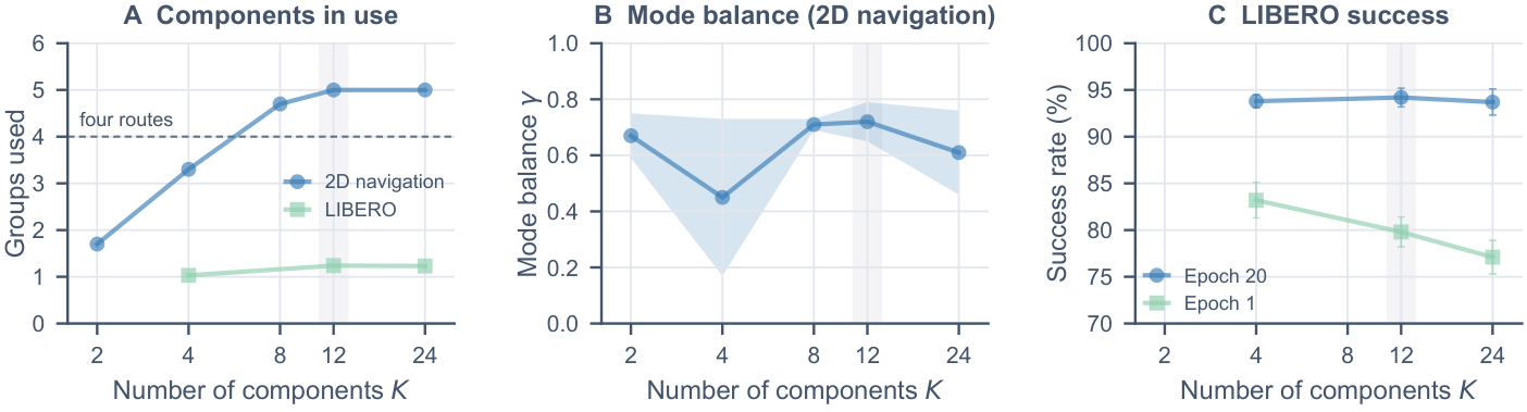
图 18:分量数的消融。(A) 多样性头在二维导航任务起点处以及在 LIBERO 每个状态上使用的不同分量组数,四条路线以虚线标出。(B) 导航任务第 20 个 epoch 的模式平衡度 \gamma。(C) LIBERO 第 1 和 20 个 epoch 的成功率(每任务 10 个回合)。三个随机种子的均值和标准差,默认 K=12 以灰色标出。
原图注:Ablation on the number of components. (A) Distinct groups of components used by the diversity head at the start of the 2D navigation task and per state on LIBERO, with the four routes as dashed line. (B) Mode balance \gamma on the navigation task at epoch 20. (C) Success rate on LIBERO at epochs 1 and 20 (10 episodes per task). Mean and standard deviation over three random seeds, with the default K=12 in gray.
图 18 解读
横轴为分量数 K\in\{2,4,8,12,24\}。 (A) 使用的分量组数:导航任务中 K=2,4,8,12,24 依次约为 1.7、3.3、4.7、5、5,K\ge8 后接近四条路线(虚线);LIBERO 中约为 1.0–1.25,即单模态任务基本只用一组。“组”指意义相近、指向同一路线的若干分量。 (B) 模式平衡度:K=2 约 0.67,K=4 约 0.45 且方差极大,K=8、12 约 0.71–0.72,K=24 约 0.61。 (C) LIBERO 成功率:第 1 个 epoch 时 K=4 约 83.2%、K=12 约 79.8%、K=24 约 77.2%;第 20 个 epoch 都在 94% 左右。 一个意外现象:K=2 只有两个分量,却得到了 0.67 的平衡度,高于 K=4。由于 \gamma>0 要求四条路线都被用到,这说明在一个分量内部采样(分量有方差)也能把路径送进不同路线,分量数并不严格等于可表达的模式数。原文没有讨论这一点。
原文
Number of components. The number of components K only bounds how many modes the diversity head can represent (Fig. 18). At K=4, the head cannot reliably separate the four routes of the navigation task, and \gamma varies strongly across seeds. From K=8 on, it uses about five groups of components at the start, close to the four routes, and about one group per state on uni-modal LIBERO. A smaller K is slightly better after one epoch, likely because the untrained head offsets the actions less, and at epoch 20 the success rate barely changes. K only needs to exceed the number of modes, and we use K=12 throughout.
译文
分量数。分量数 K 只限定多样性头能表示多少个模式(图 18)。K=4 时,多样性头无法可靠地区分导航任务的四条路线,\gamma 在不同种子间波动很大。从 K=8 起,它在起点处使用约五组分量,接近四条路线;在单模态的 LIBERO 上,每个状态约使用一组。较小的 K 在一个 epoch 后略好,可能是因为未训练好的多样性头对动作的偏移较小;到第 20 个 epoch,成功率几乎没有变化。K 只需超过模式数即可,我们全程使用 K=12。
解释
这与第 4.4 节的观察呼应:在 LIBERO 这类单模态任务上,多样性头对早期学习略有拖累(分量越多拖累越大)。作者的结论“K 只需超过模式数”在实践中需要预先估计任务的模式数,对未知任务可以取一个较大的值(如 12),代价是早期学习稍慢。
9讨论与未来方向(Discussion and Future Directions)
原文
We presented ODE policy, which models how the action of a robot evolves over its physical time as an ODE, so that each action is integrated from the previous one. In IL, it learns the vector field by integrating over short action chunks, seamless chunking joins successive chunks without jumps, and the contractive perturbation keeps the policy close to the demonstrations. On LIBERO, ODE policy reaches 79.2% after one epoch and 93.8% at epoch 100, matches FM-DiT with less than half of the demonstrations, and generates a chunk of 8 actions in 5.7 ms.
译文
我们提出了 ODE 策略,它把机器人的动作如何随其物理时间演化建模为一个 ODE,使每个动作都从前一个动作积分得到。在 IL 中,它通过在短动作块上积分来学习向量场,无缝分块使相邻动作块无跳变地衔接,收缩扰动使策略保持在示范附近。在 LIBERO 上,ODE 策略一个 epoch 后达到 79.2%,第 100 个 epoch 达到 93.8%,只用不到一半的示范就能达到 FM-DiT 的水平,并在 5.7 ms 内生成一个 8 动作块。
解释
93.8% 与第 6.1.1 节由图 4(B) 推算的 85.4+8.4=93.8 一致。5.7 毫秒是欧拉法的数字(主实验默认 RK4 约 10 毫秒)。
原文
As the action head of the \pi_{0.5} VLA, it reaches 96.0% after one epoch against 75.5% for its flow matching expert with about 3% of its parameters, and as the action head of the WAM ImageWAM, 82.6% against 24.6% for the original head, generating a chunk 4.1 times faster. On 14 real-world tasks across single-arm, dual-arm, dexterous, and humanoid robots, it achieves the highest success rate on every task, and its motion is smoother than the human demonstrations in most cases. As the actor of SuperMimic, it reaches a higher return early in training and still 0.885 against 0.845 at the end of training.
译文
作为 \pi_{0.5} VLA 的动作头,它以约 3% 的参数量在一个 epoch 后达到 96.0%,而其流匹配专家为 75.5%;作为 WAM ImageWAM 的动作头,它达到 82.6%,而原始动作头为 24.6%,生成动作块的速度快 4.1 倍。在单臂、双臂、灵巧手和人形机器人的 14 个真实任务上,它在每个任务上都取得了最高成功率,并且其运动在多数情况下比人类示范更平滑。作为 SuperMimic 的执行器,它在训练早期达到更高的回报,训练结束时仍为 0.885 对 0.845。
解释
再次提醒口径:“75.5%”是随机初始化的流匹配专家;预训练的流匹配专家在第 1 个 epoch 约 88%(图 5(A)),且在泛化测试中后期略高于 ODE(图 9(B))。“每个任务最高”中,双臂“两支花都插入”一项 ODE 只比 FM-DiT 多一次成功(2 对 1)。
原文
These results suggest that building the continuity of physical motion into the policy, rather than learning it from data, makes robot policies more efficient in learning, data, parameters, and execution, and that this gain scales from small visuomotor policies to large pretrained models and carries over from IL to RL. Beyond the results, viewing a policy as a vector field in the physical time of the robot opens uses that direct-action policies do not naturally offer. We share three aspects with preliminary experiments, as starting points rather than finished solutions, and close with a broader view of what the field may represent.
译文
这些结果表明,把物理运动的连续性内建到策略中,而不是从数据中学习它,能使机器人策略在学习、数据、参数和执行上都更高效,并且这一增益可以从小型视觉运动策略扩展到大型预训练模型,并从 IL 延续到 RL。在这些结果之外,把策略看作机器人物理时间中的向量场,还开启了直接动作策略不能自然提供的用途。我们用初步实验分享三个方面,作为起点而非完整的解决方案,最后对向量场可能代表的含义给出更宽的视角。
解释
这是全文的核心论点:归纳偏置(连续性)内建于模型结构中,比让模型从数据中学习更高效,这与 CNN 内建平移不变性、Transformer 内建置换等变性的思路一致。后面三小节(9.1–9.3)是初步实验,作者明确说是“起点而非完整方案”,单个种子、每任务 10 个回合,证据强度低于主实验。
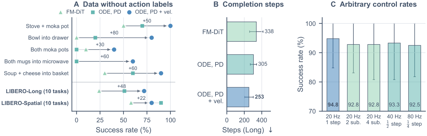
图 19:连续时间向量场的两种潜在用途。(A, B) 从没有动作标签的数据中学习。所有策略都只用 LIBERO 的实测位姿训练,在第 100 个 epoch 评测;“ODE,PD + 速度”把向量场的速度输入 PD 控制器。(A) 五个对时间要求严格的 LIBERO-Long 任务上的成功率,以及 LIBERO-Long 和 LIBERO-Spatial 上的平均成功率;(B) 成功的 Long 回合的步数。(C) 任意控制频率:对同一个训练好的模型只在部署时改变积分方式,或在 20 Hz 的每个控制步内做子步积分,或用更小的步长并发送每个中间点,以 40 或 80 Hz 运行。四个 suite 的平均成功率。单个种子,每任务 10 个回合。(A) 中的箭头给出“ODE,PD + 速度”相对 FM-DiT 的增益。(B) 和 (C) 中的须线表示任务间的标准差。
原图注:Two potential uses of the continuous-time field. (A, B) Learning from data without action labels. All policies are trained on the measured poses of LIBERO only and evaluated at epoch 100, and ODE policy with PD + velocity feeds the velocity of its field to the PD controller. (A) Success rate on five time-critical LIBERO-Long tasks and averaged over LIBERO-Long and LIBERO-Spatial, and (B) steps of successful Long episodes. (C) Arbitrary control rates, by changing the integration of one trained model at deployment, with substeps within each control step at 20 Hz or a smaller step sending every intermediate point at 40 or 80 Hz. Average success rate over the four suites. One seed with 10 episodes per task. In (A), arrows give the gain of ODE policy with PD + velocity over FM-DiT. Whiskers in (B) and (C) show the standard deviation across tasks.
图 19 解读
(A) 每行一个任务,三种标记分别为 FM-DiT(三角)、ODE + 普通 PD(方块)、ODE + PD + 速度(圆点)。五个时间敏感任务中,ODE + PD + 速度依次约为 100、80、40、60、90%,FM-DiT 约为 50、0、10、0、30%,增益 +50、+80、+30、+60、+60。底部两行为整个 suite 的平均:LIBERO-Long 中 FM-DiT 24%、ODE + PD 51%、ODE + PD + 速度 72%(+48);LIBERO-Spatial 中 FM-DiT 约 58%、ODE + PD 90%、ODE + PD + 速度 80%(相对 FM-DiT +22)。 (B) 成功的 Long 回合平均步数:FM-DiT 338,ODE + PD 305,ODE + PD + 速度 253。 (C) 五种部署方式的平均成功率:20 Hz 单步 94.8%,20 Hz 两子步 92.8%,20 Hz 四子步 92.8%,40 Hz(\frac12 步长)93.3%,80 Hz(\frac14 步长)92.5%。 要点:(A) 中速度前馈在 Long 上大幅提升,在 Spatial 上反而比普通 PD 低 10 个点,作者如实报告了这一权衡。(C) 中改变积分方式后成功率下降约 2 个点,在单种子、每任务 10 回合的统计误差范围内。
9.1从没有动作标签的数据中学习
原文
Data collected with handheld interfaces such as UMI (Chi et al., 2024) or from human videos (Kareer et al., 2026) record the measured pose but not the command sent to the controller. A policy can then only learn the measured state, which lags behind its target, so the robot moves slower than in the demonstrations (Zhao et al., 2026). Since ODE policy learns a vector field, the velocity of each action is available at no extra cost. We feed it to the damping term of the PD controller, i.e., k_p(\mathbf{p}_{\text{ref}}-\mathbf{p})+k_d(\dot{\mathbf{p}}_{\text{ref}}-\dot{\mathbf{p}}) instead of k_p(\mathbf{p}_{\text{ref}}-\mathbf{p})-k_d\dot{\mathbf{p}}, where \mathbf{p},\mathbf{p}_{\text{ref}}\in\mathbb{R}^{d_a} are the measured and reference poses and k_p,k_d\in\mathbb{R}_{>0} are the proportional and derivative gains, and train all policies on the measured poses of LIBERO only (Fig. 19(A, B)).
译文
用 UMI(Chi et al., 2024)等手持设备采集的数据或来自人类视频的数据(Kareer et al., 2026)记录的是实测位姿,而不是发送给控制器的指令。此时策略只能学习实测状态,而实测状态滞后于其目标,因此机器人的运动比示范中更慢(Zhao et al., 2026)。由于 ODE 策略学习的是向量场,每个动作的速度可以无额外代价地获得。我们把它输入 PD 控制器的阻尼项,即使用 k_p(\mathbf{p}_{\text{ref}}-\mathbf{p})+k_d(\dot{\mathbf{p}}_{\text{ref}}-\dot{\mathbf{p}}) 代替 k_p(\mathbf{p}_{\text{ref}}-\mathbf{p})-k_d\dot{\mathbf{p}},其中 \mathbf{p},\mathbf{p}_{\text{ref}}\in\mathbb{R}^{d_a} 为实测位姿和参考位姿,k_p,k_d\in\mathbb{R}_{>0} 为比例增益和微分增益;并且只用 LIBERO 的实测位姿训练所有策略(图 19(A, B))。
解释
问题:遥操作时记录的是“指令”,而 UMI(手持夹爪 + 相机)或人类视频只能记录“实际轨迹”。用实际轨迹当指令去驱动 PD 控制器,机器人会因为控制器滞后而比示范慢一拍,时间敏感的任务就会超时。 PD 控制器两种写法的区别:普通形式 -k_d\dot{\mathbf p} 是把机器人的速度往 0 拉(纯阻尼);改进形式 k_d(\dot{\mathbf p}_{\text{ref}}-\dot{\mathbf p}) 是把机器人的速度往参考速度拉,相当于加了速度前馈,机器人可以跟上运动的节奏。直接动作策略只输出位置,要得到速度只能差分,噪声大;ODE 策略的向量场本身就是速度。
原文
With the velocity, the robot keeps the demonstrated pace. Successful Long episodes take 253 instead of 305 steps, and long tasks that ran out of time are now completed, raising Long from 51% to 72% (FM-DiT: 24%). Faster motion, however, makes precise placement harder, and on Spatial the success rate drops from 90% to 80%. This hints that the velocity could be modulated by the phase of a task, e.g., fast in free space and slow near contact, which is natural to express with a vector field but hard with direct-action policies.
译文
有了速度,机器人能保持示范的节奏。成功的 Long 回合只需 253 步而不是 305 步,原先超时的长任务现在得以完成,Long 的成功率从 51% 提高到 72%(FM-DiT 为 24%)。然而,更快的运动使精确放置更难,在 Spatial 上成功率从 90% 降到 80%。这提示可以根据任务阶段调节速度,例如在自由空间中快、在接近接触时慢;这用向量场表达很自然,用直接动作策略则很难。
解释
(305-253)/305\approx17\% 的步数节省。值得注意的是:只用实测位姿训练时,FM-DiT 在 Long 上只有 24%,而 ODE 即使不加速度前馈也有 51%。这一差距本身可能来自两方面:ODE 的学习效率,以及其积分对滞后数据的某种适应。作者没有单独分析。“按阶段调节速度”是一个有意思的方向:可以在向量场上乘一个由任务阶段决定的标量,加速或减速整个运动。
9.2任意控制频率
原文
Since ODE policy is a vector field in continuous time, the integration step is a choice made at deployment rather than a part of the model. We take the model trained with one RK4 step per control step at 20 Hz and change only the integration at deployment (Fig. 19(C)). Integrating each control step with 2 or 4 substeps moves the integrated path by at most 1 mm, against about 10 mm between consecutive actions, and the success rate changes from 94.8% to 92.8%. Reducing the step to 1/2 or 1/4 and sending every intermediate point runs the same model at 40 or 80 Hz, with 16 or 32 actions per chunk, at 93.3% and 92.5% success and the same completion time.
译文
由于 ODE 策略是连续时间中的向量场,积分步长是部署时的选择,而不是模型的一部分。我们取一个以 20 Hz、每个控制步一次 RK4 步训练的模型,只在部署时改变积分方式(图 19(C))。在每个控制步内用 2 或 4 个子步积分,积分路径最多移动 1 mm,而相邻动作之间相距约 10 mm,成功率从 94.8% 变为 92.8%。把步长减为 1/2 或 1/4 并发送每个中间点,就能让同一个模型以 40 或 80 Hz 运行,每个动作块含 16 或 32 个动作,成功率为 93.3% 和 92.5%,完成时间不变。
解释
两种用法:(1) 子步积分:频率不变,只是把一步拆成几小步算,提高积分精度,路径几乎不变(最多 1 毫米),说明训练出的向量场在步与步之间是“合理”的;(2) 细化步长:每个小步都发出去,相当于把 20 Hz 的模型直接用于 40 或 80 Hz 的控制器,动作块时间长度不变(8 步 \times 1/20 秒 = 16 步 \times 1/40 秒 =0.4 秒)。成功率约下降 2 个点,在单种子小样本下难以与噪声区分。
原文
In contrast, a conventional policy outputs actions at the fixed step of its training data and must interpolate them to run at a higher rate, and even policies conditioned on physical time keep a fixed action rate (Wang et al., 2026). One model could therefore serve low-level controllers of different frequencies without retraining, and the integration step might even be adapted online, e.g., refined near contact where precise control matters most.
译文
相比之下,传统策略以其训练数据的固定步长输出动作,要以更高频率运行就必须插值,即使以物理时间为条件的策略也保持固定的动作频率(Wang et al., 2026)。因此,一个模型无需重新训练就可以服务于不同频率的底层控制器,积分步长甚至可以在线调整,例如在最需要精确控制的接触附近细化步长。
解释
对于跨本体部署很有用:不同机器人的控制频率常常不同(如 Franka 1 kHz 底层、策略 10–30 Hz),一个 ODE 策略可以适配多种频率。但要注意,提高积分频率并不提高感知频率:条件 \mathbf z_t 仍每块更新一次,所以更高的动作频率带来的是更平滑的指令,而不是更快的反应。
9.3离散动作信号
原文
An ODE describes signals that change continuously. Contact tasks nevertheless do not hurt ODE policy, e.g., 96.2% vs. 78.8% for FM-DiT at epoch 10 on eight contact-rich LIBERO tasks. The gripper command, in contrast, is binary on some robots, e.g., in LIBERO, while it is continuous on our real robots. The LIBERO experiments above predict the binary command with a separate classification head. This simple head is effective and leaves the smooth motion of the arm to the field.
译文
ODE 描述的是连续变化的信号。尽管如此,接触任务并不会损害 ODE 策略的表现,例如在八个接触丰富的 LIBERO 任务上,第 10 个 epoch 时其成功率为 96.2%,而 FM-DiT 为 78.8%。相比之下,夹爪指令在某些机器人上是二值的,例如在 LIBERO 中;而在我们的真机上则是连续的。上文的 LIBERO 实验用一个单独的分类头预测二值指令。这个简单的头很有效,并把手臂的平滑运动交给向量场。
解释
为什么接触不是问题:接触时实际位置会突然停下(被物体挡住),但指令可以继续平滑变化,由控制器的柔顺性吸收冲击。ODE 积分的是指令,所以接触不破坏其连续性假设。真正的不连续来自夹爪“开/关”这类开关量。
原文
To probe the ODE itself, we instead integrate the gripper as one more state of the field and send its sign, with each chunk starting the gripper state at the last command. Without any further design, the success rate drops from 79.2%, 95.0%, and 92.8% to 74.5%, 91.8%, and 92.2% at epochs 1, 5, and 10, mostly on Long, which requires repeated grasping and releasing. Even so, it still exceeds all baselines after one epoch (74.5% vs. at most 43.2%) and at epoch 10 (92.2% vs. at most 86.9%). Neural ODEs built for discontinuous dynamics, such as learned event functions (Chen et al., 2021a) and jump terms (Jia and Benson, 2019), might further empower ODE policy.
译文
为了检验 ODE 本身,我们改为把夹爪作为向量场的又一个状态来积分,并发送其符号,每个动作块的夹爪状态从上一次的指令开始。在不做任何额外设计的情况下,第 1、5、10 个 epoch 的成功率从 79.2%、95.0% 和 92.8% 降到 74.5%、91.8% 和 92.2%,下降主要发生在需要反复抓取和松开的 Long 上。即便如此,它在一个 epoch 后(74.5% 对最高 43.2%)和第 10 个 epoch(92.2% 对最高 86.9%)仍超过所有基线。为不连续动态设计的神经 ODE,例如学习的事件函数(Chen et al., 2021a)和跳跃项(Jia and Benson, 2019),可能进一步增强 ODE 策略。
解释
“发送其符号”:积分得到的夹爪状态是连续值,正为开、负为关。积分时它从一个符号平滑过渡到另一个符号,过零点的时刻就是开合时刻,这种方式会在过零附近带来不确定性。事件函数:神经 ODE 积分到某个条件满足时触发事件(如状态突变);跳跃项:允许状态在特定时刻不连续地跳变。这些是让 ODE 处理“开关”的成熟方法,作者留作未来工作。
原文
Actions learned without demonstrations need not be continuous either. In our early experiments with model-free RL, the learned actions often jumped between control steps, while the compliant PD controller still kept the motion smooth. There, ODE policy brought little gain and sometimes even hurt, likely because its continuity also smooths the exploration. Such jumps are, however, usually treated as a flaw rather than a need, since they load the motors and widen the gap between simulation and reality, and RL for robots commonly penalizes the change of actions (Mysore et al., 2021; Rudin et al., 2022). ODE policy thus suits best where the commands themselves should be smooth, e.g., when imitating demonstrations or deploying on hardware.
译文
在没有示范的情况下学到的动作也未必是连续的。在我们早期的无模型 RL 实验中,学到的动作常常在控制步之间跳变,而柔顺的 PD 控制器仍使运动保持平滑。在那里,ODE 策略带来的收益很小,有时甚至有害,这可能是因为它的连续性也把探索平滑化了。不过,这种跳变通常被视为缺陷而非需求,因为它会加重电机负担,并扩大仿真与现实之间的差距,机器人 RL 通常会惩罚动作的变化(Mysore et al., 2021; Rudin et al., 2022)。因此,ODE 策略最适合指令本身就应当平滑的场合,例如模仿示范或在硬件上部署。
解释
一个重要的负面结果:在 PPO 等无模型 RL 中,ODE 策略没有帮助,甚至更差。合理的解释是:无模型 RL 靠在动作上加噪声来探索,ODE 的积分会把噪声“平滑”掉,相邻步的探索噪声高度相关,探索效率降低。在 SuperMimic(基于模型、解析梯度)中则不靠随机探索,所以不受影响,反而受益于第 4.5 节所说的梯度路径。这说明 ODE 策略的 RL 优势依赖于 RL 算法的类型,不能直接推广到所有 RL 方法。
9.4动作是逐步展开的意图
原文
In physics, differential equations describe how a state changes. The action of a robot is different. It is a command, an intention of where to go next, so it is not obvious that it should follow such a law. Neuroscience suggests that it may. When a monkey reaches, its motor cortex does not simply encode the target. Its activity evolves like a dynamical system from a preparatory state, and the movement unfolds from it (Churchland et al., 2012; Shenoy et al., 2013). Human reaching is also smooth, close to minimum jerk (Flash and Hogan, 1985).
译文
在物理学中,微分方程描述状态如何变化。机器人的动作则不同:它是一条指令,是“下一步去哪里”的意图,因此并不显然应当遵循这样的规律。神经科学提示它可能确实如此。猴子伸手时,其运动皮层并不只是编码目标;它的活动从一个准备状态出发,像一个动力系统那样演化,运动由此展开(Churchland et al., 2012; Shenoy et al., 2013)。人类的伸手动作也是平滑的,接近最小加加速度(Flash and Hogan, 1985)。
解释
最小加加速度模型(minimum jerk,Flash & Hogan 1985):人手从 A 点移到 B 点的轨迹,近似于使加加速度平方积分最小的那条曲线,速度呈钟形。这是运动控制领域的经典结论。作者借此说明“平滑”是生物运动的基本特征,策略内建平滑性是合理的。
原文
ODE policy works in a similar way. At the start of each chunk, it makes a discrete choice, e.g., which arm places the apple, and the vector field then unfolds the motion. A policy might thus only need to decide at a few key points of a task, e.g., where its modes branch, and leave the rest to the learned dynamics.
译文
ODE 策略以类似的方式工作。在每个动作块开始时,它做出一个离散的选择,例如由哪只手臂放苹果,然后由向量场展开运动。因此,策略也许只需要在任务的少数关键点做决策(例如在各模式分叉的地方),其余部分交给学到的动态即可。
解释
这是一个具有启发性的展望:“稀疏决策 + 连续展开”。它与分层控制(高层选技能、底层执行)以及大模型“慢思考 + 快执行”的双系统设计(如 GR00T)思路相通。若能学到何时需要“重新决策”,策略的推理频率可以进一步降低。
致谢(Acknowledgments)
原文
We thank Sharpa Robotics for releasing the SharpaDex dataset (Sharpa Robotics, 2026), whose demonstrations we use for the cup reorientation, pill pouring, and cube stacking tasks, and for their support with the Sharpa North robot and the Sharpa hand.
译文
我们感谢 Sharpa Robotics 发布 SharpaDex 数据集(Sharpa Robotics, 2026),我们在扶杯、倒药片和叠方块任务中使用了其中的示范;并感谢他们在 Sharpa North 机器人和 Sharpa 灵巧手方面提供的支持。
解释
致谢说明了第 7.3 节跨场景实验的数据来源。
参考文献
参考文献从略,见原文。正文引用沿用原文的“作者,年份”格式,可据此在原文参考文献表中查找。A实验细节(Experimental Details)
解释
原文附录开头有一个附录目录,本译稿以总目录代替。附录中的图表编号带前缀 S(S1、S2……),以区别于正文。
原文
Simulated benchmarks. LIBERO has four suites (Object, Spatial, Goal, and Long) with 10 tasks each and 50 demonstrations per task. One model is trained on all 40 tasks and evaluated on each suite separately. LIBERO-plus perturbs the camera, the initial robot pose, the object layout, the background, the lighting, and the sensor noise. \pi_{0.5} and ImageWAM are tested on LIBERO and on a shared set of 2008 LIBERO-plus instances, which also perturb the language instruction.
译文
仿真基准。LIBERO 有四个 suite(Object、Spatial、Goal 和 Long),每个 suite 10 个任务,每个任务 50 条示范。一个模型在全部 40 个任务上训练,并在每个 suite 上分别评测。LIBERO-plus 对相机、机器人初始姿态、物体布局、背景、光照和传感器噪声施加扰动。\pi_{0.5} 和 ImageWAM 在 LIBERO 以及一组共享的 2008 个 LIBERO-plus 实例上测试,这些实例还会扰动语言指令。
解释
这里列出的视觉运动策略扰动类型是六种(不含语言),LIBERO-plus 的第七类“语言指令”扰动只用于 \pi_{0.5} 和 ImageWAM 的测试。因此视觉运动策略的 LIBERO-plus 评测共 6\times4\times50=1{,}200 个实例。
原文
Single-arm robot tasks. All four tasks on the Franka Research 3 arm use multiple cameras, and the actions are joint angles. In the box task, the arm puts a mango into a box and then closes the lid. Its 40 demonstrations are collected with a SpaceMouse through the HIL-SERL teleoperation framework (Luo et al., 2025). In the key task, the arm grasps a key and hangs it on a hook of a wooden key holder, learned from 40 demonstrations collected in the same way. In the sock task, the arm takes a sock from the top of a small cabinet, folds it on the table, puts it into the open drawer, and closes the drawer, learned from 40 demonstrations. In the insertion task, the arm grasps a blue block and inserts it into a matching hole of a black board, learned from 40 demonstrations. Inference times on this robot are measured on one RTX 5080.
译文
单臂机器人任务。Franka Research 3 机械臂上的四个任务都使用多个相机,动作为关节角。在装盒任务中,机械臂把芒果放进盒子,然后合上盖子。其 40 条示范通过 HIL-SERL 遥操作框架(Luo et al., 2025)用 SpaceMouse 采集。在挂钥匙任务中,机械臂抓起钥匙并挂到木质钥匙架的挂钩上,用同样方式采集的 40 条示范学习。在叠袜子任务中,机械臂从小柜顶部拿起一只袜子,在桌上折叠,放进打开的抽屉并关上抽屉,用 40 条示范学习。在插入任务中,机械臂抓起一个蓝色方块并插入黑色板上匹配的孔中,用 40 条示范学习。该机器人上的推理时间在一张 RTX 5080 上测量。
解释
SpaceMouse 是六自由度三维鼠标,常用于低成本遥操作;HIL-SERL 是一个人在回路的真机 RL 框架,这里只用了它的遥操作部分。动作为关节角(而 LIBERO 是末端增量),说明 ODE 策略在两种动作空间下都适用。
原文
Dual-arm robot tasks. All tasks on the dual-arm and dexterous-hand robots use joint angles as actions at 15 Hz. In the flower insertion task, one arm of the Galaxea R1 Lite grasps a long-stemmed poppy or a short-stemmed dahlia from a glass vase and inserts its thin stem into the narrow opening of another vase, so a small error of the gripper pose makes the stem miss the opening. One model is trained on both flowers from 95 demonstrations (38 poppy and 57 dahlia), with a head and a wrist camera. In the microwave task, one arm grasps a bowl of corn, places it in the microwave, and pushes it in, and the other arm then closes the door. It is learned from 34 demonstrations, with a head and two wrist cameras.
译文
双臂机器人任务。双臂和灵巧手机器人上的所有任务都以 15 Hz 的关节角作为动作。在插花任务中,Galaxea R1 Lite 的一只手臂从玻璃花瓶中抓起一支长茎罂粟花或短茎大丽花,并把其细茎插进另一个花瓶的窄口,夹爪位姿的微小误差都会使花茎错过瓶口。一个模型在两种花共 95 条示范(38 条罂粟、57 条大丽花)上训练,使用一个头部相机和一个腕部相机。在微波炉任务中,一只手臂抓起一碗玉米,放进微波炉并推到里面,另一只手臂随后关上门。它用 34 条示范学习,使用一个头部相机和两个腕部相机。
解释
罂粟只有 38 条示范,少于大丽花的 57 条,再加上茎更长,这解释了罂粟成功率(30%)明显低于大丽花(60%)。
原文
In the two-flower task, one arm inserts two flowers one after the other into the same vase, learned from 95 demonstrations. In the drawer task, one arm puts an apple from the top of a cabinet into its open drawer, and the other arm closes the drawer. The demonstrations contain both assignments of the arms, 25 with the left arm and 25 with the right arm placing the apple, with a head and two wrist cameras.
译文
在双花任务中,一只手臂把两支花先后插进同一个花瓶,用 95 条示范学习。在抽屉任务中,一只手臂把柜顶上的苹果放进打开的抽屉,另一只手臂关上抽屉。示范中包含两种手臂分配,左臂放苹果和右臂放苹果各 25 条,使用一个头部相机和两个腕部相机。
解释
抽屉任务每种模式只有 25 条示范,总共 50 条,ODE 达到 60% 成功率,模式比例 40:60。
原文
Dexterous-hand tasks. The policy runs at 15 Hz, and each predicted chunk is linearly interpolated to 60 Hz joint position targets for the arm and the 22 joints of each hand. In the can task, the Sharpa North robot picks up a can with its Sharpa hand and places it on a plate, learned from 50 demonstrations. In the cup task, the hand picks up a fallen cup, reorients it, and places it upright. Its 50 demonstrations are drawn at random from the reorient_cup_upright task of the public SharpaDex dataset (Sharpa Robotics, 2026), recorded by Sharpa in another lab, and the policies are tested in our lab with other cups and another background.
译文
灵巧手任务。策略以 15 Hz 运行,每个预测的动作块被线性插值为手臂和每只手 22 个关节的 60 Hz 关节位置目标。在罐子任务中,Sharpa North 机器人用 Sharpa 灵巧手拿起一个罐子并放到盘子上,用 50 条示范学习。在杯子任务中,灵巧手拿起倒下的杯子,把它转正并竖直放好。其 50 条示范从公开 SharpaDex 数据集的 reorient_cup_upright 任务中随机抽取,由 Sharpa 在另一个实验室录制,策略则在我们的实验室用其他杯子和另一种背景测试。
解释
插值的影响:所有方法的动作块都被线性插值到 60 Hz,因此底层看到的都是“分段线性”的轨迹。ODE 也同样被插值,并没有使用第 9.2 节的“任意频率”能力。每只手 22 个关节,加上手臂,动作维度约 30–50 维。
原文
In the pill task, the two hands pour pills from one cup into another and put both cups back. Its 50 demonstrations are those of one recording session of the transfer_pills_between_cups task of SharpaDex closest to our placement of the cups, and the policies are tested with cups of other colors. In the stacking task, the hand stacks a red cube on a green cube. Its 50 demonstrations come from the stack_cube task of SharpaDex, and the policies are tested in our lab with colored cubes instead of the wooden cubes of the demonstrations.
译文
在药片任务中,两只手把药片从一个杯子倒进另一个杯子,并把两个杯子都放回原处。其 50 条示范取自 SharpaDex 的 transfer_pills_between_cups 任务中与我们的杯子摆放位置最接近的一个录制批次,策略用其他颜色的杯子测试。在叠方块任务中,灵巧手把红色方块叠到绿色方块上。其 50 条示范来自 SharpaDex 的 stack_cube 任务,策略在我们的实验室用彩色方块代替示范中的木质方块进行测试。
解释
数据选择的细节:药片任务的示范是“与我们的摆放最接近的批次”,即作者为减小分布偏移挑选了数据;杯子任务则是随机抽取。这些选择对所有方法相同,不影响比较的公平性,但会影响“跨场景迁移”结论的强度。
原文
Humanoid tasks. The Unitree G1 humanoid with two Inspire DFX dexterous hands is controlled through GR00T N1.7 (Bjorck et al., 2025). As in ImageWAM, ODE policy reads the condition from GR00T once per chunk. A vector field of about 5M parameters, fine-tuned on top of GR00T, integrates chunks of H=16 steps with Euler, with the diversity head as in all IL experiments. The baseline is the original action head of GR00T N1.7.
译文
人形机器人任务。配备两只 Inspire DFX 灵巧手的宇树 G1 人形机器人通过 GR00T N1.7(Bjorck et al., 2025)控制。与 ImageWAM 中一样,ODE 策略每个动作块从 GR00T 读取一次条件。一个约 5M 参数的向量场在 GR00T 之上微调,用欧拉法积分 H=16 步的动作块,并与所有 IL 实验一样使用多样性头。基线是 GR00T N1.7 的原始动作头。
解释
与第 5 节相同的信息。人形任务的示范数为每任务 90 条,训练 90 个 epoch(第 7.4 节)。
原文
Visuomotor policies. All methods share the same observation encoder, a ResNet-18 (He et al., 2016) with group normalization (Wu and He, 2018) and random cropping that encodes the last 8 image frames, and a CLIP text embedding (Radford et al., 2021) of the instruction. Except in the model-size study, the parameters outside the encoder are matched to about 24M (ODE-MLP 24.40M, ODE-DiT 24.15M, FM-DiT 23.93M, and the others within 5%). All methods are trained with AdamW (Loshchilov and Hutter, 2019), learning rate 10^{-4}, batch size 32, and a cosine schedule defined over 100 epochs, and shorter runs stop early under the same schedule.
译文
视觉运动策略。所有方法共享同一个观测编码器:一个使用组归一化(Wu and He, 2018)和随机裁剪的 ResNet-18(He et al., 2016),编码最近 8 帧图像;以及指令的 CLIP 文本嵌入(Radford et al., 2021)。除模型规模研究外,编码器之外的参数量都匹配到约 24M(ODE-MLP 24.40M,ODE-DiT 24.15M,FM-DiT 23.93M,其他方法相差在 5% 以内)。所有方法都用 AdamW(Loshchilov and Hutter, 2019)训练,学习率 10^{-4},batch size 32,余弦学习率调度按 100 个 epoch 定义,较短的训练在同一调度下提前停止。
解释
“较短的训练提前停止”很关键:第 1 个 epoch 的结果是从一个 100 epoch 调度中截取的,学习率还处在高位。这对所有方法相同,所以比较公平。ResNet-18 比较小,这也解释了视觉运动策略在 LIBERO-plus 上泛化较差(约 40%)。
原文
The model-size study changes the width of the action head, with 4 layers for both methods. For the 1.5M ODE policy, the network that maps the observation features to the condition is also narrowed (condition width 136 instead of 512), since it alone has 4.2M parameters at the default width. Each visuomotor experiment is run with three random seeds, except ODE-DiT with one seed. The data-efficiency study changes only the number of demonstrations per task, so fewer demonstrations also mean fewer gradient steps per epoch.
译文
模型规模研究改变动作头的宽度,两种方法都用 4 层。对于 1.5M 的 ODE 策略,把观测特征映射为条件的网络也被缩窄(条件宽度 136 而不是 512),因为在默认宽度下仅这一网络就有 4.2M 参数。每个视觉运动实验都用三个随机种子运行,ODE-DiT 只用一个种子。数据效率研究只改变每任务的示范数,因此示范越少,每个 epoch 的梯度步数也越少。
解释
对图 4(B) 的重要补充:示范从 50 降到 5 时,每个 epoch 的梯度步数也降为 1/10。因此“第 10 个 epoch、5 条示范”时,模型实际只训练了相当于“第 1 个 epoch、50 条示范”的步数。“数据越少差距越大”的部分原因可能是训练步数更少,而 ODE 本来就在早期领先更多。若按相同梯度步数比较,差距可能会小一些。
原文
ODE policy. The vector field is a 4-layer FiLM-MLP of width 1732 that takes the action state and the proprioception as input and is modulated by the condition. It corresponds to the conditional residual block of the 1D UNet of FM-UNet and DDPM-UNet without the temporal convolution, since the field takes a single state rather than a sequence of actions, and we therefore call it ODE-MLP in the tables. ODE-DiT replaces it with AdaLN Transformer blocks of width 512 and 4 layers (Appendix B.8).
译文
ODE 策略。向量场是一个宽度为 1732 的 4 层 FiLM-MLP,以动作状态和本体感知为输入,并由条件进行调制。它对应于 FM-UNet 和 DDPM-UNet 的一维 UNet 中去掉时间卷积的条件残差块,因为向量场的输入是单个状态而不是动作序列,所以我们在表中称之为 ODE-MLP。ODE-DiT 则把它替换为宽度 512、4 层的 AdaLN Transformer 块(附录 B.8)。
解释
宽度 1732 这个不寻常的数字是为了把参数量凑到约 24M,与基线对齐。向量场是一个处理单个动作向量的 MLP,而不是处理整个动作序列,所以非常轻量,每次计算都很快。
原文
The state is the desired action of the LIBERO operational space controller, i.e., the current pose plus 0.05 m and 0.5 rad times the normalized command, so that a unit tracking gain reproduces the demonstrated command exactly. Each chunk of 8 steps is integrated with RK4 at 20 Hz. Half of the training segments are perturbed by about 1 cm and 0.03 rad with \rho=0.7. The diversity head has K=12 components. LIBERO uses the component means and the navigation task samples them. The binary gripper is predicted by a separate head.
译文
状态是 LIBERO 操作空间控制器的期望动作,即当前位姿加上 0.05 m 和 0.5 rad 乘以归一化指令,这样在单位跟踪增益下可以精确复现示范指令。每个 8 步的动作块以 20 Hz 用 RK4 积分。一半的训练片段受到约 1 cm 和 0.03 rad 的扰动,\rho=0.7。多样性头有 K=12 个分量。LIBERO 使用分量均值,导航任务则对其采样。二值夹爪由一个单独的头预测。
解释
超参数汇总:扰动概率 p=0.5,位置扰动约 1 厘米、姿态扰动约 0.03 弧度(约 1.7°),衰减率 \rho=0.7。代入公式 (7),8 步后扰动剩余 0.7^8\approx5.8\%。期望动作的换算:LIBERO 的指令是归一化到 [-1,1] 的增量,乘以 0.05 米(位置)和 0.5 弧度(姿态)就是每步的实际增量,加上当前位姿即为期望目标,这正是第 4.1 节所说的增量控制器换算。
原文
Baselines. FM-DiT, FM-UNet, DDPM-DiT, and DDPM-UNet predict chunks of 8 actions with the DiT or the 1D UNet head of the corresponding generative model. A2A-DiT starts its flow from the history of actions, perturbed by Gaussian noise of standard deviation 0.5. ACT uses its CVAE Transformer decoder. FM-DiT and FM-UNet integrate their flow with 10 midpoint steps, i.e., 20 network calls per chunk, DDPM-DiT and DDPM-UNet denoise in 100 steps, and A2A-DiT generates a chunk in one flow step. As for ODE policy, every baseline reads the last 8 image frames, predicts a chunk of 8 actions, and executes all of them before the next observation.
译文
基线。FM-DiT、FM-UNet、DDPM-DiT 和 DDPM-UNet 用对应生成模型的 DiT 或一维 UNet 头预测 8 动作块。A2A-DiT 从历史动作出发开始其流,历史动作上加有标准差为 0.5 的高斯噪声。ACT 使用其 CVAE Transformer 解码器。FM-DiT 和 FM-UNet 用 10 个中点步对流积分,即每个动作块 20 次网络计算;DDPM-DiT 和 DDPM-UNet 去噪 100 步;A2A-DiT 用一个流步生成一个动作块。与 ODE 策略一样,每个基线都读取最近 8 帧图像,预测一个 8 动作块,并在下一次观测前全部执行。
解释
推理成本的来源:FM 每块 20 次 DiT 计算,DDPM 每块 100 次,A2A 只有 1 次,ODE(RK4)每块 32 次小 MLP 计算(欧拉 8 次)。这解释了图 7(A) 中的时间排序:A2A \approx ODE(Euler) < ODE(RK4) < FM \ll DDPM。ODE 虽然计算次数不少,但每次只是一个 MLP,远比 DiT 便宜。
原文
Evaluation and metrics. Each LIBERO checkpoint runs 20 episodes for each of the 10 tasks of each suite from the fixed initial states of the benchmark. Execution quality is measured on the successful episodes. The jerk is the RMS jerk of the measured end-effector position. The in-chunk and cross-chunk smoothness are the mean change of the command between consecutive steps inside a chunk and at the first step of a new chunk, and their quotient is the boundary ratio. The completion time is the number of control steps. Inference times in the main text are measured during these evaluations on shared GPUs, and times on one idle RTX 4090 are reported in Table S1. LIBERO-plus samples 50 instances per perturbation type and suite with the same sampling seed for all methods.
译文
评测与指标。每个 LIBERO 检查点从基准固定的初始状态出发,对每个 suite 的 10 个任务各运行 20 个回合。执行质量在成功回合上测量。加加速度是实测末端位置的均方根加加速度。块内和跨块平滑度分别是动作块内部相邻步之间,以及新动作块第一步处指令的平均变化量,二者之比即边界比。完成时间是控制步数。正文中的推理时间是在共享 GPU 上评测时测得的,在一张空闲 RTX 4090 上的时间见表 S1。LIBERO-plus 对每种扰动类型和每个 suite 采样 50 个实例,所有方法使用相同的采样种子。
解释
边界比的定义:(块边界处的指令变化)/(块内的平均指令变化)。值为 1 表示边界和块内一样平滑。图 17(C) 中无缝分块约为 1.7。“共享 GPU 上测得”意味着正文中的绝对时间会受其他进程影响,相对排序更可靠,表 S1 给出了干净条件下的数字。
B补充结果(Additional Results)
B.1执行质量
原文
Table S1 repeats the timing of Fig. 7(A) on one idle RTX 4090, and the ranking stays the same. With RK4, ODE policy takes 8.82 ms per call, 4.8 times less than FM-DiT and 38 times less than DDPM-UNet, and only the single-pass ACT and A2A-DiT are faster. With Euler, it takes 4.25 ms, close to these single-pass policies. The encoder takes about 1.2 ms for every method, so the differences come from the action head. Longer chunks spread one call over more actions, and the time per action falls from 3.53 ms at H=1 to 1.09 ms at H=16.
译文
表 S1 在一张空闲的 RTX 4090 上重复了图 7(A) 的计时,排序保持不变。使用 RK4 时,ODE 策略每次调用 8.82 ms,比 FM-DiT 少 4.8 倍,比 DDPM-UNet 少 38 倍,只有单次前向的 ACT 和 A2A-DiT 更快。使用欧拉法时为 4.25 ms,接近这些单次前向策略。编码器对每种方法都约为 1.2 ms,因此差别来自动作头。更长的动作块把一次调用分摊到更多动作上,每个动作的时间从 H=1 时的 3.53 ms 降到 H=16 时的 1.09 ms。
解释
核对:42.1/8.82\approx4.8,335/8.82\approx38,与正文一致。空闲 GPU 上欧拉法相对 FM-DiT 为 42.1/4.25\approx9.9 倍,略低于正文共享 GPU 上测得的 10.8 倍。
表 S1:第 100 个 epoch 检查点在一张空闲 RTX 4090 上的推理时间(ms)。“微基准”对固定输入重复 200 次;“调用”和“动作”时间在 LIBERO-Goal 的前三个任务上闭环测得(每个任务 10 个回合),SR 为成功率(%)。参数量为全部参数(M)。
| 方法 | 微基准·调用 | 微基准·编码器 | 微基准·动作头 | 调用 | 动作 | SR | 参数量 |
| ODE-MLP(本文) | 8.82 | 1.22 | 7.6 | 9.69 | 1.25 | 96.7 | 35.6 |
| FM-DiT | 42.1 | 1.28 | 40.8 | 41.3 | 5.31 | 93.3 | 35.1 |
| FM-UNet | 58.8 | 1.22 | 57.5 | 60.1 | 7.7 | 86.7 | 36.0 |
| A2A-DiT | 3.68 | 1.24 | 2.44 | 4.79 | 0.617 | 96.7 | 35.1 |
| DDPM-DiT | 235 | 1.24 | 233 | 237 | 30.5 | 90.0 | 34.7 |
| DDPM-UNet | 335 | 1.25 | 333 | 341 | 43.5 | 93.3 | 36.0 |
| ACT | 3.19 | 1.26 | 1.94 | 4.29 | 0.549 | 80.0 | 35.2 |
| ODE-MLP,H=1 | 3.39 | 1.21 | 2.18 | 3.53 | 3.53 | 80.0 | 35.6 |
| ODE-MLP,H=4 | 6.22 | 1.28 | 4.94 | 6.86 | 1.74 | 100.0 | 35.6 |
| ODE-MLP,H=12 | 12.4 | 1.24 | 11.2 | 13.1 | 1.14 | 96.7 | 35.6 |
| ODE-MLP,H=16 | 15.8 | 1.22 | 14.5 | 16.2 | 1.09 | 100.0 | 35.6 |
| ODE-MLP,RK2 | 5.65 | 1.21 | 4.44 | 6.33 | 0.819 | 100.0 | 35.6 |
| ODE-MLP,欧拉 | 4.25 | 1.23 | 3.02 | 4.86 | 0.623 | 100.0 | 35.6 |
原表注:Inference time (ms) on one idle RTX 4090 with the epoch-100 checkpoints. Micro timings repeat a fixed input 200 times, and call and action timings are measured in closed loop on the first three tasks of LIBERO-Goal (10 episodes each), where SR is the success rate (%). Params counts all parameters (M). Unless noted, ODE-MLP uses H=8 and RK4.
表 S1 解读
列:“微基准”三列把一次调用拆成编码器和动作头两部分;“调用”和“动作”是闭环实测的每次调用时间和摊到每个动作的时间;SR 只在 LIBERO-Goal 前三个任务、每任务 10 回合上测得(共 30 次),所以 100% 与 96.7% 只差一次,不能据此比较成功率。 读法:所有方法的编码器都约 1.2 毫秒,差别全在动作头:ODE(RK4)7.6 毫秒,FM-DiT 40.8 毫秒,DDPM-UNet 333 毫秒。全部参数量(含编码器)都在 35 M 左右,说明比较的是同等规模。第二组行显示 H 越大,摊到每个动作的时间越少;第三组显示 RK2、欧拉比 RK4 更快。
B.2泛化
原文
Fig. S1 breaks the zero-shot success of the visuomotor policies on LIBERO-plus down by perturbation type at epoch 100, as summarized in Section 6.3.
译文
图 S1 把视觉运动策略在 LIBERO-plus 上第 100 个 epoch 的零样本成功率按扰动类型分解,第 6.3 节已对此做了概述。
解释
对应第 6.3.1 节“ODE 在传感器噪声下领先最多,FM-DiT 和 DDPM-DiT 更能应对初始姿态改变,相机改变使所有方法失败”的结论。
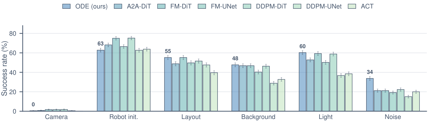
图 S1:第 100 个 epoch 时视觉运动策略在每种 LIBERO-plus 扰动类型上的零样本成功率,合并四个 suite 和三个随机种子。每组上方的数字为 ODE 策略的成功率,误差棒为合并实例上的标准误。
原图注:Zero-shot success rate of the visuomotor policies per LIBERO-plus perturbation type at epoch 100, pooled over the four suites and three random seeds. The number above each group is ODE policy, and error bars show the standard error over the pooled instances.
图 S1 解读
六组扰动,每组七根柱(ODE、A2A-DiT、FM-DiT、FM-UNet、DDPM-DiT、DDPM-UNet、ACT)。ODE 的成功率依次为:相机 0%(所有方法都接近 0)、机器人初始姿态 63%(FM-DiT 和 DDPM-DiT 约 75%,最高)、物体布局 55%(与 FM-DiT 持平,最高)、背景 48%(与多数基线相近)、光照 60%(最高,FM-DiT 约 59%)、传感器噪声 34%(其余方法 15–22%)。 要点:ODE 只在传感器噪声上明显领先,在初始姿态上落后约 12 个点,其余类型基本持平。
B.3多模态
原文
Fig. S2 shows the rollouts behind Fig. 10 for one seed. After one epoch, ODE policy already passes through all four gaps with few failures, whereas FM-DiT fails in many rollouts and mostly takes the inner routes. A2A-DiT collapses to the two inner routes throughout training. MARS covers all four routes, but many of its rollouts still fail at epoch 10.
译文
图 S2 给出了图 10 背后某个种子的推演轨迹。一个 epoch 后,ODE 策略已能穿过全部四个缺口且失败很少,而 FM-DiT 很多推演失败,且大多走内侧路线。A2A-DiT 在整个训练中都坍缩到内侧两条路线。MARS 覆盖了全部四条路线,但到第 10 个 epoch 仍有很多推演失败。
解释
这张图把图 10 的统计数字变成了可见的轨迹,是理解多模态能力最直观的材料。
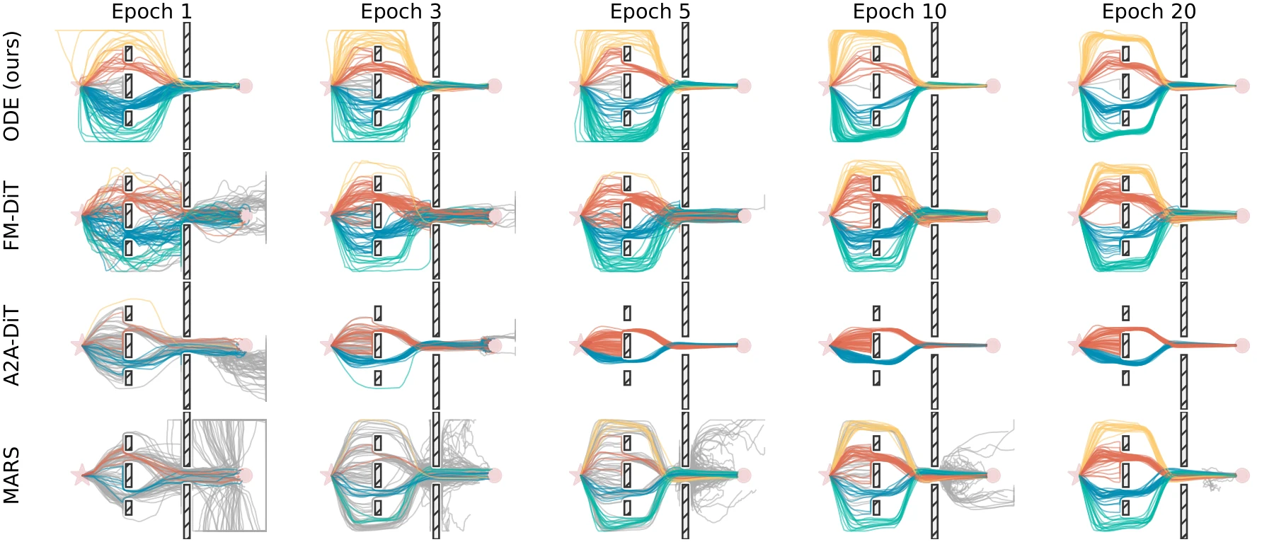
图 S2:二维导航任务在第 1、3、5、10、20 个 epoch 的推演轨迹,每格 100 条(星号为起点,圆点为目标,颜色表示经过的缺口,失败的推演为灰色)。三个随机种子之一。
原图注:Rollouts on the 2D navigation task at epochs 1, 3, 5, 10, and 20, 100 per panel (stars mark the start, circles the goal, and colors the gap taken, with failed rollouts in gray). One of the three random seeds.
图 S2 解读
四行方法 \times 五列 epoch。ODE(第一行):第 1 个 epoch 已有黄、红、蓝、青四色轨迹,少量灰色失败;之后各色轨迹越来越整齐,第 20 个 epoch 四条路线都很清晰。FM-DiT(第二行):第 1 个 epoch 有大量灰色轨迹穿墙乱走,彩色轨迹集中在中间两条;到第 10、20 个 epoch 才覆盖全部四条。A2A-DiT(第三行):自始至终只有红、蓝两条内侧路线。MARS(第四行):第 1 个 epoch 几乎全是灰色失败,第 10 个 epoch 仍有不少灰色,第 20 个 epoch 才四路齐全。
B.4视觉—语言—动作模型
原文
We fine-tune \pi_{0.5} (Physical Intelligence et al., 2025) on the four LIBERO suites jointly (1693 demonstrations) for three epochs with one seed. All parameters are trained, including the VLM of 2.92B parameters, with AdamW, a peak learning rate of 5\times10^{-5}, and a global batch size of 384 on eight A100 GPUs. Each method uses the current images of an external and a wrist camera at 224\times224 and predicts and executes chunks of 8 actions.
译文
我们在 LIBERO 四个 suite 上联合微调 \pi_{0.5}(Physical Intelligence et al., 2025)(1693 条示范),训练三个 epoch,单个种子。所有参数都参与训练,包括 2.92B 参数的 VLM,使用 AdamW,峰值学习率 5\times10^{-5},在八张 A100 GPU 上全局 batch size 为 384。每种方法都使用外部相机和腕部相机的当前图像(224\times224),预测并执行 8 动作块。
解释
1693 条示范是 LIBERO 四个 suite 去掉无效回合后的数量(原始为 2000 条)。ImageWAM 实验中为 1712 条(附录 B.5),两者略有不同,可能来自不同的数据清洗版本,原文未说明。batch 384 时一个 epoch 大约只有数百步,所以“0.5 个 epoch”已经是一个有意义的训练量。
原文
ODE policy replaces the action expert of \pi_{0.5} (430M parameters with its projections) by a learned query that reads the image and language features of the VLM once per chunk, a FiLM-MLP vector field of four residual layers of width 512, and a gripper head, 13.7M parameters in total, all randomly initialized. As in all IL experiments, it also uses the diversity head. The proprioception enters only the field and the gripper head. The field integrates each chunk with RK4 from the end of the previous one, with the contractive perturbation (1 cm and 0.03 rad, applied to half of the training chunks). FM integrates its flow with 10 Euler steps.
译文
ODE 策略把 \pi_{0.5} 的动作专家(含投影层共 430M 参数)替换为:一个每个动作块读取一次 VLM 图像和语言特征的可学习查询、一个由四个宽度为 512 的残差层组成的 FiLM-MLP 向量场,以及一个夹爪头,总计 13.7M 参数,全部随机初始化。与所有 IL 实验一样,它也使用多样性头。本体感知只输入向量场和夹爪头。向量场从前一动作块的末端出发用 RK4 积分每个动作块,并使用收缩扰动(1 cm 和 0.03 rad,作用于一半的训练动作块)。FM 用 10 步欧拉法对其流积分。
解释
\pi_{0.5} 原本的动作专家是一个与 VLM 逐层交互的 Transformer(类似 StarVLA 译稿中的 StarVLA-\pi)。ODE 头只在动作块开始时用一个查询向量“读”一次 VLM 的输出,之后的积分完全在小 MLP 中进行,因此推理极快(图 8(A) 中 2.2 毫秒)。
原文
The VLM is pretrained in all methods, and the suffix -R only marks a randomly initialized action expert. Each LIBERO checkpoint is evaluated on the 10 fixed initial states of each task, and LIBERO-plus on the shared set of 2008 instances with one episode each. The parameters of ODE policy outside the VLM are about 3% of those of the experts, so the comparison is not at matched capacity.
译文
所有方法中 VLM 都是预训练的,后缀 -R 只表示动作专家是随机初始化的。每个 LIBERO 检查点在每个任务的 10 个固定初始状态上评测,LIBERO-plus 则在共享的 2008 个实例上各评测一个回合。ODE 策略在 VLM 之外的参数量约为动作专家的 3%,因此这一比较不是在相同容量下进行的。
解释
作者明确承认“不是相同容量的比较”。容量差距对 ODE 不利,所以若 ODE 仍领先,结论更有说服力;但也意味着无法判断“同等容量的 ODE 头”会怎样。
原文
Table S2 lists the success rate per suite at epoch 1. The early lead of ODE policy over the pretrained FM expert holds in all four suites and is largest on Long (92.0% vs. 81.0%). Successful episodes of ODE policy and of the pretrained FM expert take a similar number of control steps (156.7 and 156.1).
译文
表 S2 列出了第 1 个 epoch 时各 suite 的成功率。ODE 策略相对预训练 FM 专家的早期领先在全部四个 suite 上都成立,在 Long 上最大(92.0% 对 81.0%)。ODE 策略和预训练 FM 专家的成功回合所用的控制步数相近(156.7 和 156.1)。
解释
这里补充了正文没有给出的“与预训练 FM 的比较”:第 1 个 epoch 平均 96.0% 对 88.0%,领先 8 个点。完成步数几乎相同,说明在 VLA 中 ODE 头并没有带来“更高效的运动”,这与视觉运动策略中步数减少 5–10% 的结论不同。
表 S2:\pi_{0.5} VLA 在各 LIBERO suite 上第 1 个 epoch 的成功率(%),单个种子,每任务 10 个回合。FM 从 \pi_{0.5} 预训练的动作专家开始,-R 表示随机初始化的动作专家。LIBERO-plus 为共享的 2008 个实例。
| 方法 | Spatial | Object | Goal | Long | LIBERO | LIBERO-plus |
| ODE(本文) | 96.0 | 100.0 | 96.0 | 92.0 | 96.0 | 71.5 |
| FM | 90.0 | 91.0 | 90.0 | 81.0 | 88.0 | 69.2 |
| FM-R | 83.0 | 89.0 | 71.0 | 59.0 | 75.5 | 52.6 |
原表注:The \pi_{0.5} VLA per LIBERO suite, success rate (%) at epoch 1, one seed, with 10 episodes per task. FM starts from the pretrained action expert of \pi_{0.5}, and -R marks a randomly initialized one. LIBERO-plus is the shared set of 2008 instances.
表 S2 解读
核对:三行的 LIBERO 平均均为四个 suite 的算术平均(如 FM:(90+91+90+81)/4=88.0)。读法:第 1 个 epoch 时,ODE 在每个 suite 上都最高,Long 上领先 FM 11 个点、领先 FM-R 33 个点;LIBERO-plus 上 ODE 71.5% 与 FM 69.2% 接近(差 2.3 个点),远高于 FM-R 的 52.6%。每个 suite 只有 100 次试验,相差 5 个点左右的差异在统计误差范围内。
B.5世界动作模型
原文
We fine-tune ImageWAM (Zhang et al., 2026) on the four LIBERO suites jointly (1712 demonstrations) for 10 epochs with one seed. Its image transformer (3.9B parameters) and action transformer are fine-tuned, and the text encoder is frozen. ODE policy keeps the 25 blocks of the action transformer, which read a 512-dimensional condition once per chunk through a learned query, and replaces its input, time embedding, and output layers with a FiLM-MLP vector field of four residual layers of width 512. The proprioception enters only the field.
译文
我们在 LIBERO 四个 suite 上联合微调 ImageWAM(Zhang et al., 2026)(1712 条示范),训练 10 个 epoch,单个种子。其图像 Transformer(3.9B 参数)和动作 Transformer 都参与微调,文本编码器冻结。ODE 策略保留动作 Transformer 的 25 个块,它们每个动作块通过一个可学习查询读取一次 512 维的条件;ODE 策略把动作 Transformer 的输入层、时间嵌入层和输出层替换为一个由四个宽度为 512 的残差层组成的 FiLM-MLP 向量场。本体感知只输入向量场。
解释
与 \pi_{0.5} 不同,ImageWAM 中 ODE 策略保留了原动作 Transformer 的主体(25 个块),只是让它每块运行一次、产生条件,然后由小向量场积分。原来的流匹配头要在 10 步去噪的每一步都运行这 25 个块,所以 ODE 版本推理快约 4 倍(图 8(C))。
原文
The field integrates chunks of 12 steps with Euler, with the contractive perturbation (1 cm and 0.03 rad, applied to half of the training chunks), seamless chunking, and the diversity head, and a separate head predicts the gripper. The settings that differ between the heads are listed in Table S3. LIBERO-plus uses a shared set of 2008 instances with one episode each and the same seed for all methods, and its success rate is weighted by perturbation type. All standard deviations in this subsection are over tasks, not over seeds.
译文
向量场用欧拉法积分 12 步的动作块,使用收缩扰动(1 cm 和 0.03 rad,作用于一半的训练动作块)、无缝分块和多样性头,并由一个单独的头预测夹爪。各动作头之间不同的设置列于表 S3。LIBERO-plus 使用共享的 2008 个实例,每个实例一个回合,所有方法使用相同的种子,其成功率按扰动类型加权。本小节中的所有标准差都是任务之间的,而不是种子之间的。
解释
“按扰动类型加权”:每种扰动类型的实例数不同,加权后各类型贡献相当。“标准差是任务之间的”:反映的是不同任务难度的差异,不是实验的随机误差,所以图 S3 中较宽的须线并不代表结果不稳定。
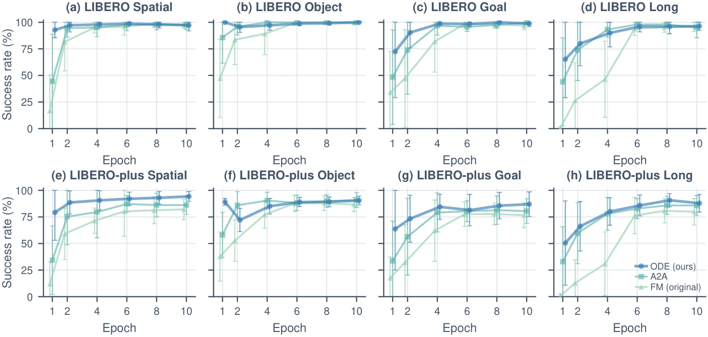
图 S3:ImageWAM 在各 LIBERO suite 上 (A-D) 以及在共享 LIBERO-plus 集合上 (E-H) 的结果,分别使用 ODE 头(本文)、A2A 头和原始流匹配头(FM)。须线表示每个 suite 十个任务之间的标准差。
原图注:ImageWAM per suite on LIBERO (A-D) and on the shared LIBERO-plus set (E-H), with the ODE head (ours), an A2A head, and the original flow matching head (FM). Whiskers show the standard deviation over the ten tasks of each suite.
图 S3 解读
上排四幅为 LIBERO 的 Spatial、Object、Goal、Long,下排为对应的 LIBERO-plus。横轴为 epoch(1–10)。LIBERO:第 1 个 epoch 时 ODE 在 Spatial 约 93%(FM 约 15%)、Object 约 100%(FM 约 47%)、Goal 约 72%(FM 约 30%)、Long 约 65%(FM 接近 0);第 4–6 个 epoch 起三者都接近 95–100%。LIBERO-plus:ODE 在 Spatial 上自始至终领先(第 10 个 epoch 约 94% 对 FM 约 80%),在其他三个 suite 上后期与 A2A 接近、略高于 FM。
表 S3:ImageWAM 中各动作头之间不同的设置。所有动作头都使用 AdamW,学习率 10^{-4},半个 epoch 的预热,余弦衰减到 10^{-6};使用两个相机的当前图像(224\times224),无图像历史,不使用 EMA;每个 epoch 是对相同数据的一次遍历。每个 LIBERO 检查点每任务评测 25 个回合。
| 设置 | FM(原始) | A2A | ODE(本文) |
| 动作生成 | 10 步流匹配 | 从历史动作出发的 1 个流步 | 读取 1 次条件,12 步欧拉 |
| 每块预测 / 执行的动作数 | 16 / 12 | 16 / 12 | 12 / 12 |
| 动作空间 | 控制器指令 | 控制器指令 | 期望动作,再换算为控制器指令 |
| 本体感知 | 条件 token | 条件 token | 向量场的输入 |
| 夹爪 | 动作流的一部分 | 动作流的一部分 | 单独的头 |
| 可训练参数 | 4517.6M | 4517.6M | 4518.2M |
原表注:ImageWAM settings that differ between the action heads. All heads use AdamW with a learning rate of 10^{-4}, a warm-up of half an epoch, and a cosine decay to 10^{-6}, the current images of two cameras at 224\times224 without image history, and no EMA, and each epoch is one pass over the same data. Each LIBERO checkpoint is evaluated with 25 episodes per task.
表 S3 解读
要点:三种动作头的可训练参数几乎相同(约 4.52B,ODE 多 0.6M),所以 ImageWAM 中的比较是相同容量的,比 \pi_{0.5} 中更公平。不过 ODE 版本同时改变了四件事:动作生成方式、动作空间(期望动作)、本体感知的位置、夹爪的处理方式。因此 ODE 的优势不能完全归因于“ODE 积分”本身,其中单独的夹爪头、本体感知输入位置等也可能有贡献。
原文
Fig. S3 shows each suite. The early lead of ODE policy is largest on Spatial and Long on LIBERO, and it lasts until epoch 10 on LIBERO-plus Spatial. Table S4 lists the success rate per perturbation type. On the full LIBERO-plus set of 10030 instances, ODE policy at epoch 10 succeeds in 88.7% of the episodes, close to its 89.9% on the shared set. The baselines were not evaluated on the full set.
译文
图 S3 给出各 suite 的结果。ODE 策略的早期领先在 LIBERO 的 Spatial 和 Long 上最大,并在 LIBERO-plus 的 Spatial 上一直持续到第 10 个 epoch。表 S4 列出了每种扰动类型的成功率。在完整的 10030 个 LIBERO-plus 实例上,ODE 策略在第 10 个 epoch 的成功率为 88.7%,与其在共享集合上的 89.9% 相近。基线没有在完整集合上评测。
解释
共享集合(2008 个)是完整集合(10030 个)的约 1/5 子集。ODE 在两者上的成绩只差 1.2 个点,说明子集有代表性。
表 S4:ImageWAM 在 LIBERO-plus 各扰动类型上的成功率(%),附任务间的标准差。左:共享的 2008 个实例,取每个动作头的最佳检查点(FM 和 A2A 为第 8 个 epoch,ODE 为第 10 个 epoch)。右:ODE 策略第 10 个 epoch 在完整的 10030 个实例上按 suite 的结果。
| 共享集合(2008) | ODE(本文),完整集合(10030) | |||||||
| 扰动 | FM | A2A | ODE | Spatial | Object | Goal | Long | 全部 |
| 相机 | 78.7\pm29.5 | 82.9\pm24.6 | 91.1\pm15.2 | 92.6\pm9.5 | 99.2\pm1.0 | 92.2\pm12.2 | 75.7\pm21.2 | 89.7\pm15.2 |
| 机器人初始姿态 | 52.5\pm26.7 | 61.6\pm24.6 | 71.7\pm22.8 | 77.1\pm11.8 | 63.3\pm11.4 | 67.0\pm17.0 | 68.7\pm13.3 | 68.8\pm14.2 |
| 语言 | 89.2\pm17.0 | 92.1\pm14.8 | 92.1\pm14.2 | 96.7\pm9.8 | 93.8\pm11.1 | 89.0\pm10.6 | 88.8\pm21.1 | 92.0\pm13.6 |
| 光照 | 97.4\pm5.9 | 95.6\pm16.2 | 98.7\pm3.7 | 99.7\pm0.9 | 100.0\pm0.0 | 94.6\pm9.5 | 96.4\pm4.4 | 97.7\pm5.2 |
| 背景 | 88.5\pm16.6 | 95.1\pm12.7 | 93.8\pm16.5 | 95.3\pm15.6 | 96.8\pm4.9 | 94.0\pm12.6 | 91.7\pm11.0 | 94.3\pm11.4 |
| 传感器噪声 | 92.9\pm11.3 | 95.6\pm10.5 | 98.3\pm4.7 | 97.7\pm3.6 | 99.1\pm2.4 | 98.2\pm3.4 | 94.4\pm7.0 | 97.3\pm4.6 |
| 物体布局 | 79.9\pm23.3 | 83.1\pm23.3 | 86.6\pm21.8 | 94.3\pm13.1 | 85.9\pm5.4 | 70.4\pm19.6 | 92.9\pm7.2 | 85.1\pm16.1 |
| 全部 | 81.9\pm10.8 | 85.8\pm10.3 | 89.9\pm8.0 | 93.2\pm4.8 | 90.5\pm2.0 | 85.4\pm7.4 | 86.1\pm7.0 | 88.7\pm6.3 |
原表注:ImageWAM on LIBERO-plus per perturbation type, success rate (%) with the standard deviation over tasks. Left, the shared set of 2008 instances at the best checkpoint of each head (epoch 8 for FM and A2A, epoch 10 for ODE). Right, ODE policy at epoch 10 on the full set of 10030 instances, per suite.
表 S4 解读
左半:共享集合上,ODE 在七类扰动中的五类最高,背景扰动上 A2A 略高(95.1 对 93.8),语言扰动上与 A2A 持平。差距最大的是相机(91.1 对 FM 78.7)和机器人初始姿态(71.7 对 52.5)。有意思的是,在视觉运动策略中,ODE 恰恰在初始姿态上落后(图 S1),在相机上所有方法都为 0;大模型中情况完全不同,说明泛化表现很大程度取决于主干。 右半:ODE 在完整集合上按 suite 分解,Spatial 最高(93.2),Goal 最低(85.4);最难的扰动仍是机器人初始姿态(68.8)。 检查点选择:每种方法取其最佳检查点(在测试集上选),对所有方法相同,但会使数字偏乐观。
B.6真实世界实验
原文
We report inference cost and smoothness on the cup task of the dexterous hand in Table S5. The baselines never succeed on this task, so their measures come from failed trials and serve only as a reference. ODE policy generates a chunk 3.4 and 5.1 times faster than FM-DiT and DDIM-UNet. Its acceleration at chunk boundaries is 0.86 times that inside chunks, close to the 0.96 of the demonstrations, whereas the baselines reach 2.03 and 2.97. Its arm jerk is about one third of that of the baselines and below that of the demonstrations, as on the can task.
译文
我们在表 S5 中报告灵巧手扶杯任务上的推理成本和平滑度。基线在这一任务上从未成功,因此它们的指标来自失败的试验,仅作参考。ODE 策略生成动作块的速度是 FM-DiT 的 3.4 倍、DDIM-UNet 的 5.1 倍。它在动作块边界处的加速度是块内的 0.86 倍,接近示范的 0.96,而两个基线分别达到 2.03 和 2.97。它的手臂加加速度约为基线的三分之一,并低于示范,与罐子任务中的情况一致。
解释
核对:35.0/10.2\approx3.4,51.8/10.2\approx5.1;手臂加加速度 6.1/19.6\approx0.31,约三分之一。边界比低于 1(0.86)意味着 ODE 在块边界处甚至比块内更平缓。基线数据来自失败试验,其动作模式(例如悬停抖动)与成功执行不同,作者对此有明确说明。
表 S5:真实扶杯任务上的推理成本与平滑度。推理时间在一张 RTX 4090 上对所有试验的所有动作块测量。平滑度在策略接管后的前 12 s 内计算,为各试验的均值 \pm 标准差。指令加速度针对 14 个手臂关节,实测运动的加加速度针对 14 个手臂关节和右手的 22 个关节。示范为来自 SharpaDex 的 50 条训练示范,切分为 8 步的动作块。
| 示范 | ODE 策略(本文) | FM-DiT | DDIM-UNet | |
| 每块时间(ms) | – | 10.2 | 35.0 | 51.8 |
| 95 分位与最大时间(ms) | – | 12.1 与 65.8 | 36.6 与 49.5 | 53.6 与 65.2 |
| 块边界加速度(rad/s^2) | 1.04 | \mathbf{0.29\pm0.06} | 6.40\pm0.82 | 10.9\pm4.5 |
| 块内加速度(rad/s^2) | 1.09 | \mathbf{0.34\pm0.06} | 3.15\pm0.10 | 4.02\pm2.30 |
| 边界/块内比 | 0.96 | 0.86 | 2.03 | 2.97 |
| 手臂加加速度(rad/s^3) | 10.3 | \mathbf{6.1\pm0.6} | 19.6\pm1.7 | 18.1\pm1.4 |
| 手部加加速度(rad/s^3) | 47 | \mathbf{37\pm15} | 62\pm8 | 49\pm6 |
原表注:Inference cost and smoothness on the real cup task. Inference is measured on one RTX 4090 over all chunks of all trials. Smoothness is computed over the first 12 s after the policy takes over, as the mean \pm standard deviation over trials. The command acceleration is taken over the 14 arm joints, and the jerk of the measured motion over the 14 arm joints and the 22 joints of the right hand. The demonstrations are the 50 training demonstrations from SharpaDex, cut into chunks of 8 steps.
表 S5 解读
读法:ODE 的指令加速度(0.29、0.34)只有示范(1.04、1.09)的约三分之一,说明它比人类示范平滑得多。一个细节:ODE 每块的最大推理时间为 65.8 毫秒,高于 FM-DiT 的最大值 49.5 毫秒,尽管其 95 分位只有 12.1 毫秒。这说明存在偶发的延迟尖峰(可能来自 GPU 调度等系统因素),原文正文和此处都没有讨论。“14 个手臂关节”说明是双臂各 7 个关节。
原文
The pill task in Table S6 gives the same picture with a baseline that also succeeds. ODE policy generates a chunk 3.5 times faster than FM-DiT. Its ratio of the acceleration at chunk boundaries to that inside chunks is 1.45, close to the 1.24 of the demonstrations, against 2.17 for FM-DiT. Its arm jerk is half of that of FM-DiT and below that of the demonstrations, while the hand jerk of both methods is close and below that of the demonstrations.
译文
表 S6 中的药片任务在有一个基线也能成功的情况下给出了同样的结论。ODE 策略生成动作块的速度是 FM-DiT 的 3.5 倍。它在动作块边界处与块内的加速度之比为 1.45,接近示范的 1.24,而 FM-DiT 为 2.17。它的手臂加加速度是 FM-DiT 的一半,并低于示范;两种方法的手部加加速度相近,且都低于示范。
解释
药片任务的基线(FM-DiT)有 50% 成功率,所以这里的比较更有意义。ODE 的边界比 1.45 高于示范(1.24),说明边界处仍有一点额外的突变,但远小于 FM-DiT。
表 S6:真实药片任务上的推理成本与平滑度。推理时间在一张 RTX 4090 上对所有试验的所有动作块测量。平滑度在策略接管后的前 12 s 内计算,为 ODE 策略 17 次成功试验和 FM-DiT 全部 20 次试验的均值 \pm 标准差。指令加速度针对 14 个手臂关节,实测运动的加加速度针对 14 个手臂关节和右手的 22 个关节。示范为来自 SharpaDex 的 50 条训练示范,切分为 8 步的动作块。
| 示范 | ODE 策略(本文) | FM-DiT | |
| 每块时间(ms) | – | 10.3 | 36.3 |
| 95 分位与最大时间(ms) | – | 12.7 与 30.5 | 42.6 与 89.4 |
| 块边界加速度(rad/s^2) | 1.57 | \mathbf{1.14\pm0.15} | 6.12\pm0.58 |
| 块内加速度(rad/s^2) | 1.27 | \mathbf{0.78\pm0.07} | 2.83\pm0.20 |
| 边界/块内比 | 1.24 | 1.45 | 2.17 |
| 手臂加加速度(rad/s^3) | 12.8 | \mathbf{9.8\pm0.6} | 19.6\pm1.5 |
| 手部加加速度(rad/s^3) | 47 | \mathbf{30\pm3} | 31\pm4 |
原表注:Inference cost and smoothness on the real pill task. Inference is measured on one RTX 4090 over all chunks of all trials. Smoothness is computed over the first 12 s after the policy takes over, as the mean \pm standard deviation over the 17 successful trials of ODE policy and all 20 trials of FM-DiT. The command acceleration is taken over the 14 arm joints, and the jerk of the measured motion over the 14 arm joints and the 22 joints of the right hand. The demonstrations are the 50 training demonstrations from SharpaDex, cut into chunks of 8 steps.
表 S6 解读
核对:36.3/10.3\approx3.5,9.8/19.6=0.5。统计口径不对称:ODE 只统计 17 次成功试验,FM-DiT 统计全部 20 次(含 10 次失败),失败试验往往包含更多犹豫和修正,可能使 FM-DiT 的平滑度指标偏差。表中“边界/块内比”一行把 ODE 的 1.45 加粗为最好,但示范的 1.24 更低,加粗只是相对 FM-DiT 而言。
B.7强化学习
原文
We build on an open-source reproduction of SuperMimic (Liao et al., 2026a). Each iteration steps 4096 simulated environments once and stores the transitions, trains the world model on them, and updates the actor by backpropagating the discounted return over 32 steps imagined in the frozen world model, plus the value of the critic at the last step. The task is whole-body tracking of the 40 complete LAFAN1 clips (2.45 hours at 50 Hz, 100 to 300 s each) with a Unitree G1 humanoid with 29 actuated joints. The action is the offset of the joint-position targets from the default pose, tracked by a PD controller.
译文
我们基于 SuperMimic(Liao et al., 2026a)的一个开源复现版本。每次迭代让 4096 个仿真环境各走一步并存储转移,用这些转移训练世界模型,然后通过在冻结的世界模型中想象 32 步并反向传播折扣回报(再加上最后一步评论家给出的价值)来更新执行器。任务是用有 29 个驱动关节的宇树 G1 人形机器人全身跟踪 40 段完整的 LAFAN1 片段(50 Hz 下共 2.45 小时,每段 100 到 300 s)。动作是关节位置目标相对默认姿态的偏移,由 PD 控制器跟踪。
解释
SuperMimic 的训练循环:真实(仿真)交互 \to 训练世界模型 \to 在世界模型中想象 32 步、用解析梯度更新执行器。“加上最后一步的价值”是为了估计 32 步之后的长期回报,这是 SVG、Dreamer 一类方法的标准做法。注意这里用的是开源复现而非原作者代码,数字可能与 SuperMimic 原论文不完全一致。
原文
The actor encodes the target motion into a latent \mathbf{z}_t\in\mathbb{R}^{32} and decodes it with 10 frames of proprioception into the action, with 8.91M parameters. We add the anchor-relative pose of BeyondMimic (Liao et al., 2026b) to the goal for both actors, since with proprioception alone the heading drifts over such long clips and the return saturates at about 0.58.
译文
执行器把目标动作编码为隐变量 \mathbf{z}_t\in\mathbb{R}^{32},再结合 10 帧本体感知解码为动作,共 8.91M 参数。我们为两种执行器都在目标中加入了 BeyondMimic(Liao et al., 2026b)的锚点相对位姿,因为仅靠本体感知时,在这么长的片段中朝向会漂移,回报会在约 0.58 处饱和。
解释
锚点相对位姿:参考动作中某个身体部位(如骨盆)相对机器人当前位置的位姿,告诉机器人“参考人物现在在你的哪个方向”。没有它,机器人只能“盲跟”关节角,长时间后会走偏。这一修改对两种执行器都加了,所以比较仍公平,但也意味着基线比原版 SuperMimic 更强。
原文
The ODE actor keeps this network and its initialization and only reads the decoder output as the velocity in Eq. (11), where the previous action is the noise-free output of the actor, so exploration noise does not accumulate along the integration. Without bounds, the integration turned an early error of the world model into a drift of the action and a collapse of the return in one of the runs. We therefore bound the change per step by 1.62 and each joint of the action by its own limit. Both bounds are set slightly above the 99th and 99.9th percentiles of the actions of converged policies of both actors, so they are rarely active.
译文
ODE 执行器保留这个网络及其初始化,只是把解码器的输出解读为公式 (11) 中的速度,其中“前一个动作”是执行器不含噪声的输出,因此探索噪声不会沿积分累积。在没有上下界的情况下,积分曾在其中一次运行中把世界模型的早期误差变成动作的漂移,并导致回报崩溃。因此,我们把每步的变化量限制在 1.62 以内,并把动作的每个关节限制在其各自的限位内。两个界都设得略高于两种执行器收敛策略动作的 99 分位和 99.9 分位,因此很少起作用。
解释
两个关键细节:(1) 积分起点用“无噪声的上一个输出”,而实际执行的动作带探索噪声。这避免了噪声通过积分不断累积成漂移,是 ODE 用于 RL 时必须注意的一点。(2) 不设上下界时出现过训练崩溃:这暴露了 ODE 形式在 RL 中的一个风险——一旦动作开始漂移,积分会让它持续偏离。作者通过设界解决,并说明界“很少起作用”。但需要注意,变化量上界只对 ODE 执行器施加,而它本身就是一种平滑约束,这与图 6(C) 中“ODE 更平滑”的结论有关。
原文
Everything else, including the world model, the critic, the rewards, the training noise, and the hyperparameters, follows the reproduction. Each run trains for 3 hours on one NVIDIA H200 GPU, about 33k iterations. Following SuperMimic, every clip is played once from its first frame with the deterministic policy and without noise or randomization, and an episode ends when the pelvis deviates from the reference beyond a threshold. We report the reward per step normalized by its maximum, averaged over all steps of each clip with the steps after a fall counted as zero and then over the 40 clips, and the mean squared second difference of the executed actions.
译文
其他一切,包括世界模型、评论家、奖励、训练噪声和超参数,都与该复现版本相同。每次运行在一张 NVIDIA H200 GPU 上训练 3 小时,约 33k 次迭代。按照 SuperMimic 的做法,每个片段用确定性策略从第一帧开始播放一次,不加噪声或随机化,当骨盆偏离参考超过阈值时回合结束。我们报告按最大值归一化的每步奖励,先对每个片段的所有步取平均(摔倒之后的步计为零),再对 40 个片段取平均;以及所执行动作的二阶差分的均方值。
解释
评测指标:归一化回报 1.0 表示每一步都完美跟踪;摔倒后计 0,所以早摔倒的片段得分很低。“二阶差分的均方值”即离散的动作加速度,对应图 6(C)。3 小时约 33k 次迭代,即每秒约 3 次迭代。
原文
PPO (Schulman et al., 2017) uses the same environment, observations, rewards, termination conditions, domain randomization, and clips as SuperMimic, but no world model. It samples its own exploration actions, so the execution noise of the environment is turned off. Its hyperparameters follow the G1 tracking configuration of BeyondMimic (Liao et al., 2026b), with 8192 parallel environments and the network size of SuperMimic. Each run also trains for 3 hours on one H200 GPU. Since an iteration of PPO differs from one of SuperMimic, all curves are plotted over wall-clock time. Fig. S4 compares the returns of the ODE actor and PPO. The training return of PPO includes its own exploration noise and is shown only for reference.
译文
PPO(Schulman et al., 2017)使用与 SuperMimic 相同的环境、观测、奖励、终止条件、域随机化和片段,但不使用世界模型。它自己采样探索动作,因此关闭了环境的执行噪声。其超参数沿用 BeyondMimic(Liao et al., 2026b)的 G1 跟踪配置,使用 8192 个并行环境和与 SuperMimic 相同的网络规模。每次运行同样在一张 H200 GPU 上训练 3 小时。由于 PPO 的一次迭代与 SuperMimic 的不同,所有曲线都以实际训练时间为横轴。图 S4 比较了 ODE 执行器和 PPO 的回报。PPO 的训练回报包含其自身的探索噪声,仅作参考。
解释
PPO 作为无模型 RL 的代表。3 小时对 PPO 来说太短(BeyondMimic 原本需要更长时间),所以 PPO 的低分主要说明“同样算力下基于模型的方法高效得多”,而不是 PPO 本身无法学会这个任务。
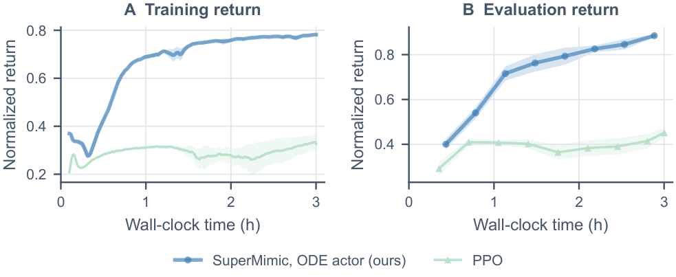
图 S4:强化学习中的回报。SuperMimic 的 ODE 执行器与 PPO 在跟踪 40 段 LAFAN1 片段的全身跟踪任务上的比较,横轴为单张 GPU 上的实际训练时间。(A) 训练回报。(B) 用确定性策略在全部 40 个片段上的归一化回报,摔倒之后的步计为零。线和阴影带为三个随机种子的均值和标准差。
原图注:Returns in reinforcement learning. The ODE actor of SuperMimic vs. PPO on whole-body tracking of the 40 LAFAN1 clips, over wall-clock time on one GPU. (A) Training return. (B) Normalized return on all 40 clips with the deterministic policy, where the steps after a fall count as zero. Lines and shaded bands show the mean and standard deviation over three random seeds.
图 S4 解读
(A) 训练回报:ODE 执行器(深蓝)在约 0.3 小时有一个短暂下降(约 0.28),随后快速上升,1 小时左右达到约 0.7,3 小时约 0.78;PPO(浅绿)一直在 0.28–0.33 之间。(B) 评测回报:ODE 从 0.4 小时的约 0.40 稳步升到 3 小时的约 0.885;PPO 在约 0.37–0.45 之间。图中没有画原始的直接动作执行器,它与 ODE 的比较见图 6。
B.8消融研究
原文
Diversity head. The head reads the features of the field with the gradient stopped, and its loss does not reach the field, so the field receives exactly the same gradient with or without the head (Section 4.4). The head thus leaves learning unchanged and only alters the actions at inference. We evaluate the same models of three seeds without the offset (\boldsymbol{\epsilon}=\mathbf{0}, i.e., the plain ODE), with the mean of the drawn component, and with full sampling within the component (Table S8).
译文
多样性头。多样性头在停止梯度的情况下读取向量场的特征,其损失不会传到向量场,因此无论有没有多样性头,向量场收到的梯度完全相同(第 4.4 节)。所以多样性头不改变学习过程,只在推理时改变动作。我们对三个种子的同一批模型,分别在不加偏移(\boldsymbol{\epsilon}=\mathbf{0},即普通 ODE)、使用抽中分量的均值,以及在分量内完全采样三种方式下进行评测(表 S8)。
解释
这是一个很干净的设计:因为向量场的训练不受多样性头影响,同一个训练好的模型可以在推理时“开关”多样性头来比较,不需要重新训练。
原文
After one epoch, when the head is not yet trained, the offset lowers the success rate from 85.3\pm1.9% to 79.8\pm1.6% with component means and to 52.1\pm0.1% with full sampling. From epoch 5 on, the three differ by at most 4.2 points, and full sampling even reaches the highest 94.8\pm0.4% at epoch 20. The diversity head therefore mainly affects the early performance, which component means largely preserve, and we use component means for uni-modal tasks.
译文
一个 epoch 后,多样性头尚未训练好,偏移使成功率从 85.3\pm1.9% 降到使用分量均值时的 79.8\pm1.6%,以及完全采样时的 52.1\pm0.1%。从第 5 个 epoch 起,三者相差最多 4.2 个百分点,完全采样在第 20 个 epoch 甚至达到最高的 94.8\pm0.4%。因此,多样性头主要影响早期性能,而使用分量均值基本保住了早期性能,我们在单模态任务上使用分量均值。
解释
重要结论:正文所有 LIBERO 结果(如“一个 epoch 后 79.2%”)都是在“分量均值”设置下得到的,比不加多样性头低约 5.5 个点。也就是说,若在单模态任务上关掉多样性头,ODE 的早期优势会更大(85.3%)。作者选择保守地报告加头的结果。“最多 4.2 个点”:第 5 个 epoch 时 95.0-90.8=4.2。
表 S7:向量场网络结构的消融,以 DiT 基线为参照。两种 ODE 变体都使用 RK4,H=8。LIBERO 上的成功率(%),对四个 suite 取平均(三个随机种子的均值,ODE-DiT 只有一个种子,每个 suite 10 个任务 \times 20 个回合);训练速度(每秒迭代次数,batch size 32);以及每个 8 动作块的推理时间(ms,共享的评测 GPU)。两种 ODE 变体在编码器外的参数量相同。
| 方法 | 向量场 | 第 1 epoch | 第 10 epoch | 第 100 epoch | it/s | ms/块 |
| ODE-MLP(本文) | FiLM-MLP | 79.2 | 93.9 | 93.8 | 17.1 | 11.0 |
| ODE-DiT(本文) | AdaLN Transformer | 77.2 | 89.6 | 91.2 | 3.5 | 51.9 |
| FM-DiT | – | 13.5 | 80.1 | 85.4 | 31.6 | 61.4 |
| A2A-DiT | – | 42.2 | 86.9 | 85.6 | 23.3 | 5.8 |
原表注:Ablation on the vector field architecture, with the DiT baselines as references. Both ODE variants use RK4 with H=8. Success rate (%) on LIBERO, averaged over the four suites (mean over three random seeds, except ODE-DiT with one seed, each suite with 10 tasks \times 20 episodes), training speed (iterations per second, batch size 32), and inference time per chunk of 8 actions (ms, shared evaluation GPUs). The two ODE variants have matched parameters outside the encoder.
表 S7 解读
这张表给出了正文中多个数字的出处:FM-DiT 第 1 个 epoch 为 13.5%(79.2/13.5\approx5.9 倍,即摘要中的倍数),A2A-DiT 第 1 个 epoch 为 42.2%(正文写“最高 43.2%”,相差 1 个点,可能来自不同的统计口径,原文未说明),ODE-MLP 第 100 个 epoch 为 93.8%,FM-DiT 为 85.4%。 训练速度:ODE-MLP 每秒 17.1 次迭代,比 FM-DiT(31.6)慢约 46%,因为 RK4 每块要在训练时算 32 次向量场并反向传播。也就是说,ODE 的“学得快”是按 epoch 计的;按实际训练时间计,优势要打折扣,但 ODE 第 2 个 epoch 就达到 85%,FM-DiT 要 30 个 epoch,即使每步慢近一倍,按图 16(D) 的训练时长换算(RK4 每 epoch 约 0.23 小时、FM-DiT 约 0.16 小时),达到 85% 的墙钟时间仍快约 10 倍。 ODE-DiT:换成 Transformer 向量场后仍超过所有基线,但比 MLP 版本差、慢得多(3.5 it/s,51.9 毫秒/块)。
原文
Vector field architecture. We replace the FiLM-MLP vector field with AdaLN Transformer blocks of FM-DiT, keeping the number of parameters (ODE-DiT, Table S7). With the Transformer, ODE policy still outperforms all baselines, with 77.2% after one epoch and 91.2% at epoch 100 (one seed), against at most 43.2% and 87.8%, and it exceeds FM-DiT with the same blocks by 5.8 points at epoch 100. However, it stays below the MLP field at every checkpoint and is much slower, training at 3.5 instead of 17.1 iterations per second and taking 51.9 instead of 11.0 ms per chunk (Table S9).
译文
向量场网络结构。我们在保持参数量不变的情况下,把 FiLM-MLP 向量场替换为 FM-DiT 的 AdaLN Transformer 块(ODE-DiT,表 S7)。使用 Transformer 时,ODE 策略仍超过所有基线:一个 epoch 后为 77.2%,第 100 个 epoch 为 91.2%(单个种子),而基线最高分别为 43.2% 和 87.8%;在第 100 个 epoch,它比使用相同块的 FM-DiT 高 5.8 个百分点。然而,它在每个检查点都低于 MLP 向量场,而且慢得多:训练速度为每秒 3.5 次迭代而不是 17.1 次,每个动作块需要 51.9 ms 而不是 11.0 ms(表 S9)。
解释
核对:91.2-85.4=5.8。“基线最高 87.8%”指第 100 个 epoch 所有基线中的最高值;表 S7 只列了 FM-DiT(85.4)和 A2A-DiT(85.6),原文未指明 87.8% 属于哪个基线,从图 4(A) 看应是某个扩散基线。这个消融有力地说明:优势来自 ODE 形式本身,而不是 MLP 结构。
原文
Two reasons explain this. First, RK4 evaluates the field 32 times per chunk, in training as well as in execution, so the overhead of each Transformer call is multiplied. Second, the Transformer of FM-DiT models the dependencies among the actions of a chunk, whereas in ODE policy the integration already produces the chunk step by step, and the field only maps the current state to its velocity, a low-dimensional mapping that an MLP fits well. A simple MLP field is therefore sufficient, as the integration carries the temporal structure of the chunk.
译文
原因有二。第一,RK4 每个动作块要计算 32 次向量场,训练和执行时都是如此,因此每次 Transformer 调用的开销被成倍放大。第二,FM-DiT 的 Transformer 建模的是动作块内各动作之间的依赖关系,而在 ODE 策略中,积分已经一步步地产生了动作块,向量场只需把当前状态映射为其速度,这是一个低维映射,MLP 就能很好地拟合。因此,简单的 MLP 向量场就足够了,因为积分承担了动作块的时间结构。
解释
第二点是对 ODE 策略本质的精炼概括:时间结构交给积分,网络只学局部映射。这也解释了为什么 ODE 策略参数效率高(图 4(C)):网络要学的东西本身就简单。
表 S8:推理时多样性头的作用,同一批模型。不加偏移(\boldsymbol{\epsilon}=\mathbf{0},普通 ODE)、使用抽中分量的均值,以及在分量内完全采样。四个 LIBERO suite 的平均成功率(%),三个随机种子的均值 \pm 标准差,括号内为各 suite 均值(Object / Spatial / Goal / Long),每任务 10 个回合。
| 推理方式 | 第 1 epoch | 第 5 epoch | 第 10 epoch | 第 20 epoch |
| 不加偏移 | 85.3\pm1.9 (98/81/91/72) | 95.0\pm1.0 (99/97/96/87) | 92.8\pm1.0 (99/94/93/85) | 93.1\pm1.2 (99/97/93/84) |
| 分量均值(本文) | 79.8\pm1.6 (98/78/83/60) | 94.8\pm0.4 (100/97/96/87) | 94.3\pm1.3 (99/98/95/86) | 94.2\pm1.0 (99/95/95/87) |
| 完全采样 | 52.1\pm0.1 (79/50/52/28) | 90.8\pm0.0 (96/94/90/82) | 93.7\pm1.1 (98/93/96/87) | 94.8\pm0.4 (99/99/94/87) |
原表注:The diversity head at inference, for the same models. Without the offset (\boldsymbol{\epsilon}=\mathbf{0}, the plain ODE), with the mean of the drawn component, and with full sampling within the component. Success rate (%) averaged over the four LIBERO suites, mean\pmstd over three random seeds, with the per-suite means in parentheses (Object / Spatial / Goal / Long), and 10 episodes per task.
表 S8 解读
读法:第 1 个 epoch 时完全采样只有 52.1%,Long 仅 28%,说明未训练好的多样性头给出的随机偏移严重干扰了动作。分量均值主要损失在 Long(72 \to 60)和 Goal(91 \to 83)。第 10、20 个 epoch 时,加了多样性头的两种方式反而略高于不加偏移(94.3、94.8 对 92.8、93.1),差距在 1–2 个点,处于种子间波动范围附近。 核对:括号内四个 suite 的均值与总体均值大致相符(如分量均值第 1 epoch:(98+78+83+60)/4=79.75)。注意括号内的 suite 顺序为 Object / Spatial / Goal / Long,与正文其他地方的 Spatial / Object / Goal / Long 不同。
表 S9:向量场网络结构的消融。两种 ODE 变体都使用 RK4,H=8。LIBERO 上的执行质量和推理时间,统计所有 suite 和种子的成功回合(回合间的均值 \pm 标准差)。SR 为三个随机种子成功率的均值和标准差。块内和跨块分别为动作块内部相邻步之间以及新动作块第一步处指令的平均变化量。Jerk 为实测末端位置的均方根加加速度(m/s^3)。Steps 为成功回合的控制步数,时间为单个种子每个动作和每次调用的推理时间(ms),在共享评测 GPU 上测得。ODE-DiT 只用一个种子训练。
| 方法 | Ep. | SR | 块内 | 跨块 | Jerk | Steps | ms/动作 | ms/调用 |
| ODE-MLP(本文) | 20 | 92.9\pm0.5 | \mathbf{0.01871}\pm0.0051 | \mathbf{0.02855}\pm0.0059 | \mathbf{5.257}\pm2.1 | \mathbf{146.5}\pm71 | \mathbf{1.43}\pm0.079 | \mathbf{11.11}\pm0.55 |
| 50 | 93.8\pm0.3 | \mathbf{0.0196}\pm0.0053 | \mathbf{0.0257}\pm0.0054 | \mathbf{5.577}\pm2.3 | \mathbf{146}\pm70 | \mathbf{1.432}\pm0.072 | \mathbf{11.15}\pm0.56 | |
| 100 | 93.8\pm1.3 | \mathbf{0.02017}\pm0.0054 | \mathbf{0.02453}\pm0.0053 | \mathbf{5.736}\pm2.3 | 147.2\pm72 | \mathbf{1.414}\pm0.069 | \mathbf{11}\pm0.47 | |
| ODE-DiT(本文) | 20 | 89.4 | 0.01914\pm0.005 | 0.02893\pm0.0057 | 5.276\pm2.1 | 148.5\pm73 | 7.192\pm0.23 | 55.97\pm1.3 |
| 50 | 90.8 | 0.02058\pm0.0052 | 0.02596\pm0.0059 | 5.734\pm2.3 | 146.6\pm73 | 7.155\pm0.26 | 55.63\pm1.5 | |
| 100 | 91.2 | 0.02133\pm0.0053 | 0.02516\pm0.0057 | 5.942\pm2.3 | \mathbf{144.5}\pm69 | 6.672\pm0.19 | 51.91\pm0.92 |
原表注:Ablation on the vector field architecture. Both ODE variants use RK4 with H=8. Execution quality and inference time on LIBERO, over the successful episodes of all suites and seeds (mean \pm standard deviation over episodes). SR is the mean and standard deviation of the success rate over three random seeds. In-chunk and cross-chunk denote the mean change of the command between consecutive steps inside a chunk and at the first step of a new chunk. Jerk is the RMS jerk of the measured end-effector position (m/s^3). Steps is the number of control steps of a successful episode, and time is the inference time per action and per call (ms) of one seed, measured on shared evaluation GPUs. ODE-DiT is trained with one seed.
表 S9 解读
读法:两种结构的平滑度(块内、跨块、Jerk)和完成步数非常接近,差别主要在成功率(约低 2–3 个点)和速度(慢约 5 倍)。跨块/块内之比:ODE-MLP 在第 20、50、100 个 epoch 分别为 0.02855/0.01871\approx1.53、1.31、1.22,随训练逐渐接近 1,与图 17(C) 中约 1.6–1.8 的边界比大致一致。Jerk 随训练上升:ODE-MLP 从 5.26 升到 5.74,这在图 7(B) 中已经出现,原文没有解释,可能是训练后期向量场学到了示范中更多的细节(包括抖动)。
译者附注:原文数字核对与阅读提示汇总
以下各条已在正文对应位置的解释框中说明,这里集中列出。总体而言,本文数字自洽程度较高:表 S2 的平均值、各真机成功率与正文的试验次数、表 S1/S5/S6 中的倍数、RL 回报比值等,按原文数据重算均一致。需要注意的主要是对比口径和实验设置。| 位置 | 说明 |
| 摘要 / 引言 | 5.9 倍成功率(79.2 对 13.5)、5.4 倍泛化(30.1 对约 5.6)、3.9 倍模式平衡(0.54 对 0.14)都是第 1 个 epoch 与 FM-DiT 的比值;训练充分后差距小得多。 |
| 引言 / 第 9 节 | “96.0% 对其流匹配专家的 75.5%”中,75.5% 是随机初始化的专家;预训练专家第 1 个 epoch 为 88.0%(表 S2)。 |
| 图 9(B) | \pi_{0.5} 中,1.5 个 epoch 之后预训练 FM 在 LIBERO-plus 上的成绩高于 ODE(约 78% 对 71%);正文只与随机初始化版本比较。 |
| 第 6.2 节 | “快 10.8 倍”为欧拉法、共享 GPU;主实验默认 RK4,空闲 GPU 上为 4.8 倍(欧拉约 9.9 倍)。 |
| 表 S7 / 图 16(D) | ODE(RK4)训练速度 17.1 it/s,FM-DiT 31.6 it/s;训练到 100 个 epoch 分别为 22.8 和 16.3 小时。正文“训练时间相当”指欧拉法。 |
| 第 4.4 节 / 表 S8 | 多样性头使 LIBERO 第 1 个 epoch 成功率从 85.3% 降到 79.8%;正文结果均为加头后的数字。 |
| 第 6.1.1 节 | 正文称 A2A-DiT 第 1 个 epoch 约 43.2%,表 S7 为 42.2%。 |
| 图 4(B) / 附录 A | 示范越少,每个 epoch 的梯度步数越少;“数据越少差距越大”部分来自训练步数的差异。 |
| 图 8(B) / 图 17(C) | 无缝分块下边界比仍约 1.5–2,位置连续但变化速率在条件刷新时仍有跳变。 |
| 第 6.1.3 节 / 附录 B.7 | RL 中只有 ODE 执行器加了每步变化量上界(1.62);不设上界时曾有一次训练崩溃;最终回报只高 4.7%(0.885 对 0.845)。 |
| 第 9.3 节 | 早期无模型 RL 实验中 ODE 策略几乎无益甚至有害,作者推测是连续性平滑了探索。 |
| 图 16 | H=16 的第三个种子训练发散;H\ge12 时出现损失尖峰。 |
| 图 7(B) / 表 S9 | ODE 的末端加加速度随训练上升(约 5.26 \to 5.74),而多数基线随训练下降,后期差距缩小。 |
| 第 7.1 节 | 单臂真机只训练 50 个 epoch,衡量早期效果。 |
| 第 7.2 节 | “两支花都插入”ODE 2/20 对 FM-DiT 1/20,是“每个任务最高”中最弱的一项。 |
| 表 S5 / 表 S6 | 扶杯任务中基线指标来自失败试验;药片任务中 ODE 只统计成功试验、FM-DiT 统计全部;扶杯任务 ODE 最大延迟 65.8 ms 高于基线最大值。 |
| 表 S3 | ImageWAM 中 ODE 版本同时改变了动作生成、动作空间、本体感知位置和夹爪处理四项,优势不能完全归因于积分本身。 |
| 表 S4 | 各方法取在测试集上选出的最佳检查点。 |
| 图 18(B) | K=2 的模式平衡度(0.67)高于 K=4(0.45),分量数与可表达模式数并非一一对应;原文未讨论。 |
| 附录 B.4 / B.5 | \pi_{0.5} 实验用 1693 条示范,ImageWAM 实验用 1712 条,原文未说明差别来源。 |